It is seldom the case that all the data we need exists in one dataset from the beginning. Usually, we have to put together several datasets to get all the variables we want in one dataset. This process is called joining dataset (also known as merging). We’ll learn about left_join, right_join, inner_join and full_join to join datasets. However, joining datasets can be quite tricky. Sometimes, the codes might not run and it can be difficult to understand why, and sometimes, the code might run and the result becomes utterly wrong. Therefore, we need to have a good overview of what exactly the two datasets show.
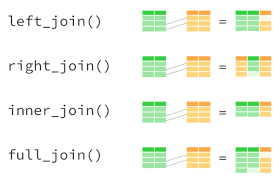
There are four main types of joins in R:
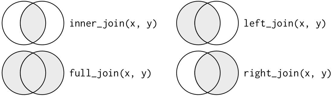
inner_joinleft_joinright_joinfull_joinWhich one to use depends on which rows it is important to keep onwards. If you only want the units that match perfectly on the variables the two datasets have in common, use inner_join. If you want to keep all units in the dataset on the left side, use left_join, and if it is more important to maintain the units in the dataset on the right side, use right_join. full_join keeps all units.
We’ll join the costofliving dataset with a dataset on welfare institutions.
Let’s first have a look at the costofliving dataset. Recall from earlier that this is a dataset that tracks the cost of living by cities in 2022, gathered from [this website](https://www.kaggle.com/datasets/kkhandekar/cost-of-living-index-by-city-2022).
costofliving <- readRDS("../datafolder/costofliving2.rds")
head(costofliving)
# A tibble: 6 × 8
city country cofi rent_index cost_of_living_plus_…¹ groceries_index
<chr> <chr> <dbl> <dbl> <dbl> <dbl>
1 Zurich Switzer… 131. 69.3 102. 136.
2 Lugano Switzer… 124. 45.0 87.0 129.
3 Bergen Norway 100. 34.8 69.7 96.2
4 Trondheim Norway 99.4 37.7 70.5 95.1
5 Reykjavik Iceland 97.6 46.3 73.6 91.9
6 Tel Aviv-Yafo Israel 94.5 53.2 75.2 83.0
# ℹ abbreviated name: ¹cost_of_living_plus_rent_index
# ℹ 2 more variables: restaurant_price_index <dbl>,
# local_purchasing_power_index <dbl>Now we want to merge this dataset with a dataset on welfare institutions.
You can find the welfare dataset here and the codebook here. Because the dataset has 400 variables to begin with, it’s a good idea to use the codebook to check which variables you might need and select these into a smaller dataset.
The dataset is in .xlsx format. To read in this type of data, we can load the package readxl and use the function read_excel. Then we can use select to fetch the variables we want and make a smaller dataset (often called a subset).
library(readxl)

welfare <- read_excel("../datafolder/CWS-data-2020.xlsx")

welfare_subset <- welfare %>%
  select(id, year, mgini, ngini, rred, lowpay)
Now, If we want to join these two datasets we first need to have a look at some necessary steps first.
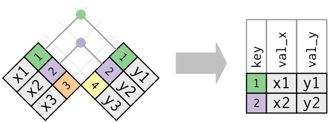
The first thing to tackle is the so-called key of the datasets. The key is the variable or variables in the two datasets that are the same. Often, it is for example an id of a person, a country name and/or a time period such as a date or a year. In our case, there’s only one shared key between the datasets – country.
The key needs to have the same values. Here, we bump into another issue. The variables indicating the countries in the welfare_subset and the costofliving datasets struggle with two problems to be a shared key: (1) the variables are called different things (id in welfare_subset and country in costofliving), and (2) they have different labels for the same values (e.g. Australia is AUS in welfare_subset but Australia in costofliving).
To change this, we could use case_when together with mutate and recode every value.
welfare_subset %>%
  mutate(country = case_when( # Make a new variable called country
    id == "AUS" ~ "Australia", # When the variable id is "AUS", give the country variable value "Australia"
    id == "BEL" ~ "Belgium",
    id == "CAN" ~ "Canada"
  ))
# A tibble: 1,299 × 7
id year mgini ngini rred lowpay country
<chr> <dbl> <dbl> <dbl> <dbl> <dbl> <chr>
1 AUL 1960 NA NA NA NA <NA>
2 AUL 1961 NA NA NA NA <NA>
3 AUL 1962 NA NA NA NA <NA>
4 AUL 1963 NA NA NA NA <NA>
5 AUL 1964 NA NA NA NA <NA>
6 AUL 1965 NA NA NA NA <NA>
7 AUL 1966 NA NA NA NA <NA>
8 AUL 1967 40.6 28.5 NA NA <NA>
9 AUL 1968 40.6 28.4 NA NA <NA>
10 AUL 1969 40.6 28.4 NA NA <NA>
# ℹ 1,289 more rowsThis is a bit time consuming, so we’ll use a shortcut here through the countrycode package. This package gives a standardized framework to recode country variables into new values (as you might understand, different values on country variables has been a pain for many joining problems).
library(countrycode)

welfare_subset <- welfare_subset %>%
  mutate(country = countrycode(sourcevar = id, # Use the id variable to find the country name
                                 origin = "iso3c", # The inital variable has three letters for countries, also called the iso3c standard
                                 destination = "country.name")) # Recode these into full country names (in English)
Warning: There was 1 warning in `mutate()`.
ℹ In argument: `country = countrycode(sourcevar = id, origin = "iso3c",
destination = "country.name")`.
Caused by warning in `countrycode_convert()`:
! Some values were not matched unambiguously: AUL, DEN, FRG, GRE, IRE, NET, POR, SPA, UKMThe warning message tells us that R was unable to translate all the values. Usually, we might want to look further into this and perhaps manually recode these variables (e.g. using case_when). However, since I won’t use this data in any analysis today, I’ll simply proceed to the joining.
One last thing that need to be done, is to remove whitespace from the country variable in costofliving. See more about this in the part on strings.
costofliving <- costofliving %>%
mutate(country = str_squish(country))When we join datasets, what we want to to add variables to the units we already have. So, in this case, we would like to add variables on redistribution to the cost of living in different cities. But there’s a problem. Even though city is our smallest units in the costofliving dataset, it is not present in the welfare_subset dataset. Here, the smallest units are countries.
glimpse(costofliving)Rows: 187
Columns: 8
$ city <chr> "Zurich", "Lugano", "Bergen", "Trondhei…
$ country <chr> "Switzerland", "Switzerland", "Norway",…
$ cofi <dbl> 131.24, 123.99, 100.38, 99.43, 97.61, 9…
$ rent_index <dbl> 69.26, 44.99, 34.84, 37.74, 46.27, 53.2…
$ cost_of_living_plus_rent_index <dbl> 102.19, 86.96, 69.66, 70.52, 73.55, 75.…
$ groceries_index <dbl> 136.14, 129.17, 96.22, 95.11, 91.92, 82…
$ restaurant_price_index <dbl> 132.52, 119.80, 103.51, 103.21, 105.77,…
$ local_purchasing_power_index <dbl> 129.79, 111.96, 86.96, 88.00, 74.84, 70…glimpse(welfare_subset)Rows: 1,299
Columns: 7
$ id <chr> "AUL", "AUL", "AUL", "AUL", "AUL", "AUL", "AUL", "AUL", "AUL",…
$ year <dbl> 1960, 1961, 1962, 1963, 1964, 1965, 1966, 1967, 1968, 1969, 19…
$ mgini <dbl> NA, NA, NA, NA, NA, NA, NA, 40.6, 40.6, 40.6, 40.5, 40.5, 40.4…
$ ngini <dbl> NA, NA, NA, NA, NA, NA, NA, 28.5, 28.4, 28.4, 28.3, 28.1, 28.0…
$ rred <dbl> NA, NA, NA, NA, NA, NA, NA, NA, NA, NA, NA, NA, NA, NA, NA, 31…
$ lowpay <dbl> NA, NA, NA, NA, NA, NA, NA, NA, NA, NA, NA, NA, NA, NA, NA, 11…
$ country <chr> NA, NA, NA, NA, NA, NA, NA, NA, NA, NA, NA, NA, NA, NA, NA, NA…Since we cannot break the country variable in the welfare_subset dataset down to cities (because we simply do not know which part of the variables belong to which cities), we have to go the other way and aggregate the variables in the costofliving dataset up to country level. We can do this through summarise and mean, as shown below. I use mean instead of sum because it doesn’t make that much sense to add up index values. Now, we find the average cost of living in each country compared to New York, based on their biggest cities.
costofliving_agg <- costofliving %>%
  group_by(country) %>% # Find the following statistic per country
  summarise(cofi = mean(cofi, na.rm = TRUE), # The average cost of living based on the biggest cities in that country
            rent_index = mean(rent_index, na.rm = TRUE),
            groceries_index = mean(groceries_index, na.rm = TRUE),
            restaurant_price_index = mean(restaurant_price_index, na.rm = TRUE),
            local_purchasing_power_index = mean(local_purchasing_power_index, na.rm = TRUE))
Alternatively, if you want to be a bit more advanced and do it with less code, you can use summarise_at and make a function.
costofliving %>%
  group_by(country) %>%
  summarise_at(vars("cofi", "rent_index", "groceries_index", "restaurant_price_index", "local_purchasing_power_index"),
               function(x){mean(x, na.rm = TRUE)}) # This function is equivalent to the one above, but with less lines of code
# A tibble: 65 × 6
country cofi rent_index groceries_index restaurant_price_index
<chr> <dbl> <dbl> <dbl> <dbl>
1 Albania 38.7 11.3 31.0 29.9
2 Argentina 35.2 10.7 28.5 34.4
3 Australia 79.2 41.8 78.3 73.6
4 Austria 69.4 33.4 64.4 67.7
5 Bangladesh 35.1 6.21 31.5 24.4
6 Botswana 42.7 11.8 35.7 52.2
7 Brazil 36.7 11.5 31.5 29.1
8 Bulgaria 42.2 14.6 36.7 38.8
9 Canada 71.9 34.1 71.7 66.8
10 China 48.7 31.3 52.8 34.7
# ℹ 55 more rows
# ℹ 1 more variable: local_purchasing_power_index <dbl>Another thing to consider is the time aspect. Our welfare_subset data has data from 1960 to 2018. Our costofliving dataset has only data from 2022. In theory, we cannot really merge the datasets then, because we do not know the cost of living in any of the years of the welfare data, and vice versa. However, doing a rough approximation, we can pick a late year in the welfare_subset dataset with sufficiently complete values and assume that the variables do not change enough from year to year, so that within a ten-year period, it should correspond more or less.
welfare_subset <- welfare_subset %>%
  filter(year == 2015) %>% # Filtering out the value on year that is 2015
  select(-year) # Removing the variable year since it now only has one value, 2015
Now we can begin to join the datasets.
The left_join function is the most used, possibly because it’s more intuitive. You start with a dataset, keep all the rows, and add variables from another dataset to the rows you already have. Here, I use left_join, keeping all the units in the costofliving_agg dataset, and join by the variable “country” which both datasets have key is country – to specify this, add by = "country".
costofliving_agg %>%
  left_join(welfare_subset, by = "country")  %>%
  select(country, cofi, rent_index, id, mgini, ngini)# I select only a few variables from each dataset so it's easier for you to see
# A tibble: 65 × 6
country cofi rent_index id mgini ngini
<chr> <dbl> <dbl> <chr> <dbl> <dbl>
1 Albania 38.7 11.3 <NA> NA NA
2 Argentina 35.2 10.7 <NA> NA NA
3 Australia 79.2 41.8 AUS 48.3 27.8
4 Austria 69.4 33.4 <NA> NA NA
5 Bangladesh 35.1 6.21 <NA> NA NA
6 Botswana 42.7 11.8 <NA> NA NA
7 Brazil 36.7 11.5 <NA> NA NA
8 Bulgaria 42.2 14.6 <NA> NA NA
9 Canada 71.9 34.1 CAN 46 30.9
10 China 48.7 31.3 <NA> NA NA
# ℹ 55 more rowsNow we have a dataset with all units from the costofliving_agg dataset and the matched units from the welfare_subset dataset. However, many NA are generated from using left_join. That’s because values on the country variable such as NY and HI are not shared between the two datasets. What we get is 162 rows with lots of missing. If we use a right_join, we lose many of these rows – now we only have 22 – but they mostly have full data.
costofliving_agg %>%
  right_join(welfare_subset, by = "country") %>%
  select(country, cofi, rent_index, id, mgini, ngini)
# A tibble: 22 × 6
country cofi rent_index id mgini ngini
<chr> <dbl> <dbl> <chr> <dbl> <dbl>
1 Australia 79.2 41.8 AUS 48.3 27.8
2 Canada 71.9 34.1 CAN 46 30.9
3 France 71.0 23.9 FRA 49.2 29.5
4 Italy 68.0 21.9 ITA 50 33.5
5 Japan 85.6 42.7 JPN NA NA
6 New Zealand 73.8 34.7 NZL 47.1 33.4
7 Norway 99.9 36.3 NOR 45.4 25.8
8 Sweden 74.9 29.2 SWE 51.5 26.4
9 United States 72.9 46.5 USA 50.6 37.9
10 <NA> NA NA AUL NA NA
# ℹ 12 more rowsNow we have a dataset with all units from the welfare_subset dataset and the matched units from the costofliving_aggdataset.
Using inner_join keeps only the rows where the values can be matched between the two datasets. Now, we have lots of information (less missing), but only 11 rows.
costofliving_agg %>%
  inner_join(welfare_subset, by = "country") %>%
  select(country, cofi, rent_index, id, mgini, ngini)
# A tibble: 9 × 6
country cofi rent_index id mgini ngini
<chr> <dbl> <dbl> <chr> <dbl> <dbl>
1 Australia 79.2 41.8 AUS 48.3 27.8
2 Canada 71.9 34.1 CAN 46 30.9
3 France 71.0 23.9 FRA 49.2 29.5
4 Italy 68.0 21.9 ITA 50 33.5
5 Japan 85.6 42.7 JPN NA NA
6 New Zealand 73.8 34.7 NZL 47.1 33.4
7 Norway 99.9 36.3 NOR 45.4 25.8
8 Sweden 74.9 29.2 SWE 51.5 26.4
9 United States 72.9 46.5 USA 50.6 37.9Last, full_join keeps all units, matching the ones it can match and adding missing values to the rest. This dataset contains 173 rows5.
costofliving_agg %>%
  full_join(welfare_subset, by = "country") %>%
  select(country, cofi, rent_index, id, mgini, ngini)
# A tibble: 78 × 6
country cofi rent_index id mgini ngini
<chr> <dbl> <dbl> <chr> <dbl> <dbl>
1 Albania 38.7 11.3 <NA> NA NA
2 Argentina 35.2 10.7 <NA> NA NA
3 Australia 79.2 41.8 AUS 48.3 27.8
4 Austria 69.4 33.4 <NA> NA NA
5 Bangladesh 35.1 6.21 <NA> NA NA
6 Botswana 42.7 11.8 <NA> NA NA
7 Brazil 36.7 11.5 <NA> NA NA
8 Bulgaria 42.2 14.6 <NA> NA NA
9 Canada 71.9 34.1 CAN 46 30.9
10 China 48.7 31.3 <NA> NA NA
# ℹ 68 more rowsMarket (Pre-Tax-and-Transfer) GINI Coefficient. Household income, whole population.↩︎
Net (Post-Tax-and-Transfer) GINI Coefficient Household income, whole population.↩︎
Relative Redistribution; market-income inequality minus net-income inequality, divided by market-income inequality. Household income, whole population.↩︎
Defined as the percentage of workers earning less than two thirds of the median wage↩︎
This is composed of 162 rows from the costofliving_agg dataset plus 22 rows from the welfare_subset dataset, minus the 11 rows that they share↩︎