21 Example solutions
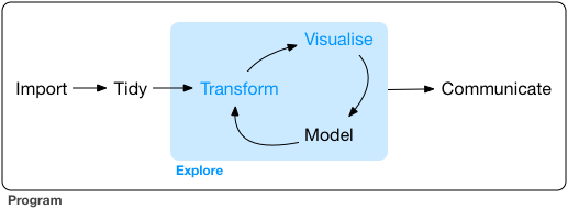
This worksheet is centered around the workflow in the picture below. Using the example research question below, we are going to see how one can go from having data and a question, to perhaps finding some answers.
Research question: Is there a positive correlation between minimum wage and your experienced financial security, in EU-countries from 2015 until 2020?
Task: Fill in the blank spaces (___) in the code.
21.1 Importing data
First, we need to install and library in the necessary packages.
# eval: false
install.packages("eurostat") # Installing the package "eurostat"
Installing eurostat [3.8.2] ...
OK [linked cache]Eurostat is the statistical office of the European Union. They have made their own R-package which we can use to gather data directly from their database with the use of code. For a full overview of their database, see this link.
library(eurostat)
library(tidyverse)
We use the function get_eurostat() to upload data from the Eurostat package to R. Make sure you are connected to wifi when you run the code.
Fetch the datasets shown below and give the datasets we upload the following names: unexp, pop, and minwage.
unexp <- get_eurostat("ilc_mdes04") # Percentage of population with inability to face unexpected financial expenses
pop <- get_eurostat("demo_pjan") # Population on 1 January by age and sex
minwage <- get_eurostat("earn_mw_cur") # Monthly minimum wages - bi-annual data
21.2 Tidy and transform
21.2.1 1. Get an overview of the data
head(unexp) # Printing the six first rows of the dataset unexp.# A tibble: 6 × 6
hhtyp incgrp unit geo time values
<chr> <chr> <chr> <chr> <date> <dbl>
1 A1 A_MD60 PC AT 2022-01-01 20.5
2 A1 A_MD60 PC BE 2022-01-01 25.5
3 A1 A_MD60 PC BG 2022-01-01 44.4
4 A1 A_MD60 PC CY 2022-01-01 35.6
5 A1 A_MD60 PC CZ 2022-01-01 21.5
6 A1 A_MD60 PC DE 2022-01-01 32.8glimpse(unexp) # Have a look at the type of variables, and the number of rows and columns in the dataset unexp.Rows: 35,734
Columns: 6
$ hhtyp <chr> "A1", "A1", "A1", "A1", "A1", "A1", "A1", "A1", "A1", "A1", "A1…
$ incgrp <chr> "A_MD60", "A_MD60", "A_MD60", "A_MD60", "A_MD60", "A_MD60", "A_…
$ unit <chr> "PC", "PC", "PC", "PC", "PC", "PC", "PC", "PC", "PC", "PC", "PC…
$ geo <chr> "AT", "BE", "BG", "CY", "CZ", "DE", "DK", "EA20", "EE", "EL", "…
$ time <date> 2022-01-01, 2022-01-01, 2022-01-01, 2022-01-01, 2022-01-01, 20…
$ values <dbl> 20.5, 25.5, 44.4, 35.6, 21.5, 32.8, 25.4, 31.2, 26.1, 53.9, 32.…head(pop) # Printing the six first rows of the dataset pop.# A tibble: 6 × 6
unit age sex geo time values
<chr> <chr> <chr> <chr> <date> <dbl>
1 NR TOTAL F AL 2022-01-01 1406532
2 NR TOTAL F AT 2022-01-01 4553444
3 NR TOTAL F AZ 2022-01-01 5081846
4 NR TOTAL F BE 2022-01-01 5883978
5 NR TOTAL F BG 2022-01-01 3527626
6 NR TOTAL F CH 2022-01-01 4400588glimpse(pop) # Have a look at the type of variables, and the number of rows and columns in the dataset pop.Rows: 713,818
Columns: 6
$ unit <chr> "NR", "NR", "NR", "NR", "NR", "NR", "NR", "NR", "NR", "NR", "NR…
$ age <chr> "TOTAL", "TOTAL", "TOTAL", "TOTAL", "TOTAL", "TOTAL", "TOTAL", …
$ sex <chr> "F", "F", "F", "F", "F", "F", "F", "F", "F", "F", "F", "F", "F"…
$ geo <chr> "AL", "AT", "AZ", "BE", "BG", "CH", "CY", "CZ", "DE", "DE_TOT",…
$ time <date> 2022-01-01, 2022-01-01, 2022-01-01, 2022-01-01, 2022-01-01, 20…
$ values <dbl> 1406532, 4553444, 5081846, 5883978, 3527626, 4400588, 463622, 5…head(minwage) # Printing the six first rows of the dataset minwage# A tibble: 6 × 4
currency geo time values
<chr> <chr> <date> <dbl>
1 EUR AL 2023-01-01 298.
2 EUR BE 2023-01-01 1955.
3 EUR BG 2023-01-01 399.
4 EUR CY 2023-01-01 940
5 EUR CZ 2023-01-01 717.
6 EUR DE 2023-01-01 1987 glimpse(minwage) # Have a look at the type of variables, and the number of rows and columns in the dataset minwage.Rows: 5,258
Columns: 4
$ currency <chr> "EUR", "EUR", "EUR", "EUR", "EUR", "EUR", "EUR", "EUR", "EUR"…
$ geo <chr> "AL", "BE", "BG", "CY", "CZ", "DE", "EE", "EL", "ES", "FR", "…
$ time <date> 2023-01-01, 2023-01-01, 2023-01-01, 2023-01-01, 2023-01-01, …
$ values <dbl> 297.65, 1955.04, 398.81, 940.00, 717.37, 1987.00, 725.00, 831…names(pop) # Put one of the datasets into this function, what does the function tell us about the dataset?[1] "unit" "age" "sex" "geo" "time" "values"# We see the variable names (column names) in the datasetnrow(unexp) # Put another dataset into this function, what does the function tell us about the dataset?[1] 35734# We see the number of observations (number of rows) in the dataset. 21.2.2 2. Missing values
unexp %>%
  complete.cases() # Print a table that shows us all units with missing values on at least one variable.
minwage %>%
select(values) %>% # Get the variable "values" from the dataset.
is.na() %>%
table() # Count the number of units which are missing on the variable "values"..
FALSE TRUE
3746 1512 21.2.3 3. Are the variables useful?
The time-variable
table(unexp$time) # Print the values of the variable "time" from the dataset "unexp".
2003-01-01 2004-01-01 2005-01-01 2006-01-01 2007-01-01 2008-01-01 2009-01-01
       357        765       1530       1581       1734       1734       1734
2010-01-01 2011-01-01 2012-01-01 2013-01-01 2014-01-01 2015-01-01 2016-01-01
      1887       2040       2040       2142       2142       2176       2142
2017-01-01 2018-01-01 2019-01-01 2020-01-01 2021-01-01 2022-01-01
2193 2244 2091 1938 1785 1479 - What does this variable tell us? Is it useful?
- Is it important for us to know that the data is for the 1st of January each year, or only that its valid for that year?
- Do we need data for all years? (see the research question at the top of the script)
unexp_reduced <- unexp %>% # change the variable "time" with the function ifelse() so it only contains the year, and not the date.
  mutate(time = ifelse(time == "2015-01-01", "2015",
                       ifelse(time == "2016-01-01", "2016",
                              ifelse(time == "2017-01-01", "2017",
                                     ifelse(time == "2018-01-01", "2018",
                                            ifelse(time == "2019-01-01", "2019",
                                                   ifelse(time == "2020-01-01", "2020",
                                                          time))))))) %>%
filter(time %in% c("2015", "2016", "2017", "2018", "2019", "2020")) # Get the rows with the years 2015, 2016, 2017, 2018, 2019 and 2020. table(unexp_reduced$time) # Check if your code is correct. Remember that we have now made a new dataset with a new name.
2015 2016 2017 2018 2019 2020
2176 2142 2193 2244 2091 1938 table(pop$time) # Check if the dataset "pop" has it's time-variable coded the same way as in the dataset unexp.
1960-01-01 1961-01-01 1962-01-01 1963-01-01 1964-01-01 1965-01-01 1966-01-01
      6836       7101       6804       6804       6804       7096       6804
1967-01-01 1968-01-01 1969-01-01 1970-01-01 1971-01-01 1972-01-01 1973-01-01
      6810       7168       7171       7512       8162       7842       8415
1974-01-01 1975-01-01 1976-01-01 1977-01-01 1978-01-01 1979-01-01 1980-01-01
      8409       8697       8425       8731       8731       8863       9145
1981-01-01 1982-01-01 1983-01-01 1984-01-01 1985-01-01 1986-01-01 1987-01-01
      8940       9510       8931       9180       9480       9789       9786
1988-01-01 1989-01-01 1990-01-01 1991-01-01 1992-01-01 1993-01-01 1994-01-01
      9789       9879      10155      10431      10493      11654      11959
1995-01-01 1996-01-01 1997-01-01 1998-01-01 1999-01-01 2000-01-01 2001-01-01
     12157      12111      12160      12113      12445      12855      13692
2002-01-01 2003-01-01 2004-01-01 2005-01-01 2006-01-01 2007-01-01 2008-01-01
     14037      13999      14005      13975      16020      16041      16311
2009-01-01 2010-01-01 2011-01-01 2012-01-01 2013-01-01 2014-01-01 2015-01-01
     16326      16059      16185      16138      16029      15900      15858
2016-01-01 2017-01-01 2018-01-01 2019-01-01 2020-01-01 2021-01-01 2022-01-01
     15900      16209      16284      16254      14127      14432      13890
# A more efficient approach to getting only the year from the "date" variable
pop_reduced <- pop %>%
mutate(time = substr(time, 1, 4)) # Make a new variable "time" in the dataset "pop" with only year, not datepop_reduced <- pop_reduced %>%
filter(time %in% c("2015", "2016", "2017", "2018", "2019", "2020")) # Get only the years we needThe minwage-dataset is different. It is biannual, which means that it’s for every other year.
table(minwage$time)
1999-01-01 1999-07-01 2000-01-01 2000-07-01 2001-01-01 2001-07-01 2002-01-01
       105        106        107        107        107        107        107
2002-07-01 2003-01-01 2003-07-01 2004-01-01 2004-07-01 2005-01-01 2005-07-01
       108        108        108        108        108        108        108
2006-01-01 2006-07-01 2007-01-01 2007-07-01 2008-01-01 2008-07-01 2009-01-01
       108        108        108        108        108        108        108
2009-07-01 2010-01-01 2010-07-01 2011-01-01 2011-07-01 2012-01-01 2012-07-01
       108        108        108        108        108        105        105
2013-01-01 2013-07-01 2014-01-01 2014-07-01 2015-01-01 2015-07-01 2016-01-01
       108        111        111        111        111        111        111
2016-07-01 2017-01-01 2017-07-01 2018-01-01 2018-07-01 2019-01-01 2019-07-01
       111        111        111        111        111        111        111
2020-01-01 2020-07-01 2021-01-01 2021-07-01 2022-01-01 2022-07-01 2023-01-01
       111        111        108        108        101         80         80
Since the other datasets we have are for years, this dataset also need to be in years for us to compare them. Therefore we get the rows with minimum wage for the 1st of January.
# Make sure the following code is in the right order:
minwage_reduced <- minwage %>%
  mutate(time = as.character(time)) %>%
  filter(!time %in% c("2020-07-01", "2019-07-01", "2018-07-01", "2017-07-01", "2016-07-01", "2015-07-01")) %>%
  mutate(time = substr(time, 1, 4)) %>%
  filter(time %in% c("2015", "2016", "2017", "2018", "2019", "2020"))
The value-variable
class(unexp_reduced$values) # Find the class of the variable "values" in the unexp-dataset. Comment what the class is. [1] "numeric"# numeric max(unexp_reduced$values, na.rm = TRUE) # Find the maximum value of the variable "values" in the dataset unexp.[1] 100min(unexp_reduced$values, na.rm = TRUE) # Find the minimum value of the variable "values" in the dataset unexp.[1] 0What does this variable tell us?
head(unexp_reduced)# A tibble: 6 × 6
hhtyp incgrp unit geo time values
<chr> <chr> <chr> <chr> <chr> <dbl>
1 A1 A_MD60 PC AL 2020 52.2
2 A1 A_MD60 PC AT 2020 17.2
3 A1 A_MD60 PC BE 2020 24.1
4 A1 A_MD60 PC BG 2020 55.2
5 A1 A_MD60 PC CH 2020 19.3
6 A1 A_MD60 PC CY 2020 30.2table(unexp_reduced$unit)
   PC
12784
Run the code above and look at the variable “unit”. It has the value “PC”. This indicates that the variable “values” is given in percentage. So the “values” show the percentage in each EU-country (“geo”) who says that they could not manage a sudden financial cost (according to household type (“hhtyp”) and income group (“incgrp”)).
Is “values” a useful name for the variable?
unexp_reduced <- unexp_reduced %>%
  rename(unexp_percent = values) # Change the name of the variable from "values" to "unexp_percent".
Check if the datasets pop and minwage also have variables called “values”.
glimpse(pop_reduced) # What type of value do you think the "values"-variable is given in? Comment below. Rows: 94,632
Columns: 6
$ unit <chr> "NR", "NR", "NR", "NR", "NR", "NR", "NR", "NR", "NR", "NR", "NR…
$ age <chr> "TOTAL", "TOTAL", "TOTAL", "TOTAL", "TOTAL", "TOTAL", "TOTAL", …
$ sex <chr> "F", "F", "F", "F", "F", "F", "F", "F", "F", "F", "F", "F", "F"…
$ geo <chr> "AL", "AM", "AT", "AZ", "BE", "BG", "CH", "CY", "CZ", "DE", "DE…
$ time <chr> "2020", "2020", "2020", "2020", "2020", "2020", "2020", "2020",…
$ values <dbl> 1425342, 1562689, 4522292, 5039100, 5841215, 3581836, 4337170, …table(pop_reduced$unit)
   NR
94632
# NR - which stands for numberglimpse(minwage_reduced)Rows: 666
Columns: 4
$ currency <chr> "EUR", "EUR", "EUR", "EUR", "EUR", "EUR", "EUR", "EUR", "EUR"…
$ geo <chr> "AL", "AT", "BE", "BG", "CH", "CY", "CZ", "DE", "DK", "EE", "…
$ time <chr> "2020", "2020", "2020", "2020", "2020", "2020", "2020", "2020…
$ values <dbl> 213.45, NA, 1593.81, 311.89, NA, NA, 574.62, 1544.00, NA, 584…table(minwage_reduced$currency)
EUR NAC PPS
222 222 222
# EUR, NAC and PPS. Different currencies. Change the name of these variables as well.
pop_reduced <- pop_reduced %>%
  rename(n_people = values)
minwage_reduced <- minwage_reduced %>%
rename(minwage_eur = values) 21.2.4 4. Are the observations useful?
What are the units in our research question? Which variable differentiate between the units in the dataset unexp? Comment below.
glimpse(unexp_reduced)Rows: 12,784
Columns: 6
$ hhtyp <chr> "A1", "A1", "A1", "A1", "A1", "A1", "A1", "A1", "A1", "A…
$ incgrp <chr> "A_MD60", "A_MD60", "A_MD60", "A_MD60", "A_MD60", "A_MD6…
$ unit <chr> "PC", "PC", "PC", "PC", "PC", "PC", "PC", "PC", "PC", "P…
$ geo <chr> "AL", "AT", "BE", "BG", "CH", "CY", "CZ", "DE", "DK", "E…
$ time <chr> "2020", "2020", "2020", "2020", "2020", "2020", "2020", …
$ unexp_percent <dbl> 52.2, 17.2, 24.1, 55.2, 19.3, 30.2, 23.6, 36.2, 25.6, 31…# EU-countries, they are in the geo-variable.
# The units are grouped by two variables: hhtyp og incgrp. Which values are in the hhtyp-variable (household type)?
table(unexp_reduced$hhtyp)
      A_GE3   A_GE3_DCH          A1      A1_DCH     A1_GE65     A1_LT65
        752         752         752         752         752         752
        A1F         A1M          A2     A2_1DCH     A2_2DCH    A2_2LT65
        752         752         752         752         752         752
A2_GE1_GE65   A2_GE3DCH      HH_DCH     HH_NDCH       TOTAL
        752         752         752         752         752
Which values are in the incgrp-variable (income group)?
table(unexp_reduced$incgrp)
A_MD60 B_MD60  TOTAL
  4250   4250   4284
Get only the row with the value “TOTAL” from the incgrp-variable.
unexp_reduced <- unexp_reduced %>%
  filter(incgrp == "TOTAL")
Get from the hhtyp-variable only the rows with the values “A1F”, “A1M”, “A2” and “TOTAL”.
unexp_reduced <- unexp_reduced %>%
  filter(hhtyp %in% c("A1F", "A1M", "A2", "TOTAL"))
Now the variables “incgrp” and “unit” have the same values, and therefore does not give us more useful information. Remove the variables “incgrp” and “unit” from the dataset.
unexp_reduced <- unexp_reduced %>%
  select(hhtyp, geo, time, unexp_percent)
We tidy the pop-dataset and the minwage-dataset in the same way. Fill in the code below so it’s correct.
pop_reduced <- pop_reduced %>%
  filter(age == "TOTAL") %>%
  filter(sex == "T") %>%
  select(geo, time, n_people)
minwage_reduced <- minwage_reduced %>%
filter(currency == "EUR") %>%
select(-(currency)) # Minus with select() removes the variables21.2.5 5. Descriptive statistics
Find the average percentage who says that they could manage a sudden financial cost.
mean(unexp_reduced$unexp_percent, na.rm = TRUE) [1] 39.18611Change the variable n_people (population size) to log.
log(pop_reduced$n_people) [1] 14.86141 14.90060 16.00168 16.12478 16.25981 15.75447 15.96797 13.69673
[9] 16.18519 18.23636 18.23636 15.57729 19.64332 19.65152 14.09992 20.06173
[17] 20.06956 16.48111 16.18749 17.67271 20.05048 19.91878 15.52485 18.02497
[25] 15.12839 15.21624 16.09478 15.41781 12.80528 17.90386 10.56481 14.84302
[33] 13.34728 14.46140 13.34049 14.54608 13.15108 16.67242 15.49589 17.45199
[41] 16.14726 16.77711 15.75089 16.15033 14.55548 15.51257 18.23622 17.54680
[49] 18.02058 14.39331 11.24081 14.86718 14.90248 15.99692 16.11624 16.25398
[57] 15.76143 16.06419 15.96080 13.68301 16.18105 18.23458 18.23458 15.57442
[65] 19.64071 19.64893 14.09679 20.05917 20.06706 16.47354 16.18805 17.66432
[73] 20.04799 19.91683 20.05597 15.52351 18.02285 15.13016 15.22069 16.09511
[81] 15.40561 12.78547 17.90679 10.55524 14.84305 13.32758 14.46782 13.34099
[89] 14.54650 13.10940 16.66519 15.48853 17.45238 16.14538 16.78153 15.75623
[97] 16.14085 14.54831 15.51120 18.22228 17.55279 18.01492 14.40089 14.86994
[105] 14.90499 15.99279 16.10785 16.24900 15.76854 16.06594 15.95371 13.66960
[113] 16.17731 18.23185 18.23185 15.57012 19.63987 19.64813 14.09249 20.05785
[121] 20.06580 16.46638 16.18959 17.65836 20.04673 19.91630 20.05478 15.52264
[129] 18.02059 15.13182 15.22784 16.09568 15.39044 12.76125 17.91789 10.54834
[137] 14.84830 13.30802 14.47530 13.34127 14.54562 13.07254 16.65932 15.48239
[145] 17.45248 16.14678 16.78764 15.76163 16.13005 14.54155 15.50986 10.44735
[153] 18.20762 17.55833 18.00930 14.40247 14.87212 14.90950 15.98717 16.09891
[161] 16.24488 15.77587 16.06730 15.94607 13.65863 16.17436 18.22857 18.22857
[169] 15.56450 19.63765 19.64605 14.08983 20.05551 20.06358 16.45842 16.19211
[177] 17.65557 20.04446 19.91479 20.05262 15.52086 18.01736 15.12875 15.23963
[185] 16.09764 15.38087 12.73183 17.91963 10.54033 14.86209 13.28901 14.48340
[193] 15.08270 13.34132 14.54485 13.03963 16.65351 15.47532 17.45238 16.14858
[201] 16.79328 15.76716 16.11761 14.54107 15.50843 18.19522 17.56301 18.00280
[209] 14.39411 14.87177 14.91365 15.97889 16.08822 16.24130 15.78315 16.06663
[217] 15.93503 13.65101 16.17200 18.22437 18.22437 15.55725 19.63530 19.64383
[225] 14.09006 20.05300 20.06116 16.44797 16.19355 17.65367 20.04203 19.91314
[233] 20.05028 15.51795 18.01479 15.12934 15.24837 16.10100 15.36865 12.71448
[241] 17.92089 10.53534 14.87627 13.26430 14.49301 13.34105 14.54368 13.01792
[249] 16.64749 15.46623 17.45223 16.15166 16.79920 15.77227 16.10309 14.54025
[257] 15.50676 18.18168 17.56715 17.99571 14.38740 14.87531 14.91765 15.96552
[265] 16.07655 16.23475 15.78990 16.06479 15.92423 13.64947 16.17052 18.21240
[273] 18.21240 15.54888 19.63155 19.64022 14.08925 20.04958 20.05784 16.43805
[281] 16.20041 17.65388 20.03867 19.91058 20.04702 15.51511 18.01208 15.13178
[289] 15.25660 16.10355 15.35830 12.70412 17.92303 10.52852 14.88753 13.24096
[297] 14.50168 15.08391 13.34085 14.54266 12.99383 16.64287 15.45770 17.45324
[305] 16.15489 16.80475 15.77763 16.09251 14.53961 15.50586 18.16831 17.57111
[313] 17.98764Find the average percentage who says they could not manage a sudden financial cost, grouped by year and country
unexp_reduced %>%
  group_by(geo, time) %>%
  summarise(unexp_pc_mean = mean(unexp_percent))
`summarise()` has grouped output by 'geo'. You can override using the `.groups`
argument.# A tibble: 252 × 3
# Groups: geo [46]
geo time unexp_pc_mean
<chr> <chr> <dbl>
1 AL 2017 62.4
2 AL 2018 57.1
3 AL 2019 55.0
4 AL 2020 48.6
5 AT 2015 24.3
6 AT 2016 24.7
7 AT 2017 23.7
8 AT 2018 22.6
9 AT 2019 20.8
10 AT 2020 19.0
# ℹ 242 more rows21.3 Visualize
Make a boxsplot with unexp_percent (percentage with financial insecurity) on the x-axis. geo (country) on the y-axis and colour by hhtyp (household type). What does this plot tell us?
unexp_reduced %>%
  ggplot(aes(x = unexp_percent, y = geo, color = hhtyp)) +
geom_boxplot() 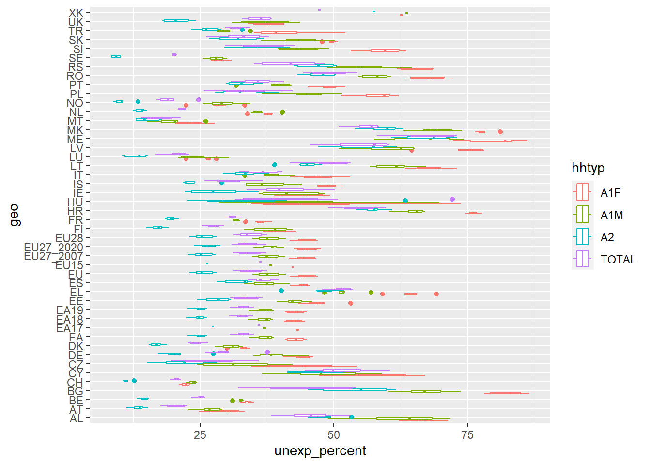
The plot shows us the percentage who says they could not manage a sudden financial cost over the year 2015-2020 according to country. The line in the middle shows the median of the percentage, the box indicates the 1st quantile and the 3rd quantile, and the line is the data’s “range”. The dots are outliers, and the boxes have different colours according to type of household.
Filter out only the countries FR (France), DE (Germany), ES (Spain), BE (Belgium), NO (Norway), SE (Sweden) and DK (Denmark), then plot again. Recode the values on the hhtyp to something that is more understandable.
unexp_reduced %>%
  filter(geo %in% c("FR", "DE", "ES", "BE", "NO", "SE", "DK")) %>%
  mutate(hhtyp = ifelse(hhtyp == "A1F", "Single women",
                        ifelse(hhtyp == "A1M", "Single men",
                               ifelse(hhtyp == "A2", "Two adults", hhtyp)))) %>%
  ggplot(aes(x = unexp_percent, y = geo, color = hhtyp)) +
geom_boxplot() 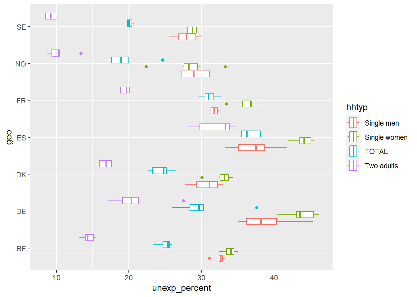
Which country has the highest percentage who reports financial insecurity? - Spain
Which country has the lowest percentage who reports financial insecurity? - Norway
Which type of household has the highest percentage who reports financial insecurity? - Single women
What is the approximate median of the percentage who reports financial insecurity among households with two adults in Germany? - 20 percent
Plot the minimum wage for the European countries over time with a line diagram. Colour the dots by country.
minwage_reduced %>%
  ggplot(aes(x = time, y = minwage_eur, group = geo, color = geo)) +
  geom_line() +
  labs(x = "", y = "Minimum wage")
Warning: Removed 54 rows containing missing values (`geom_line()`).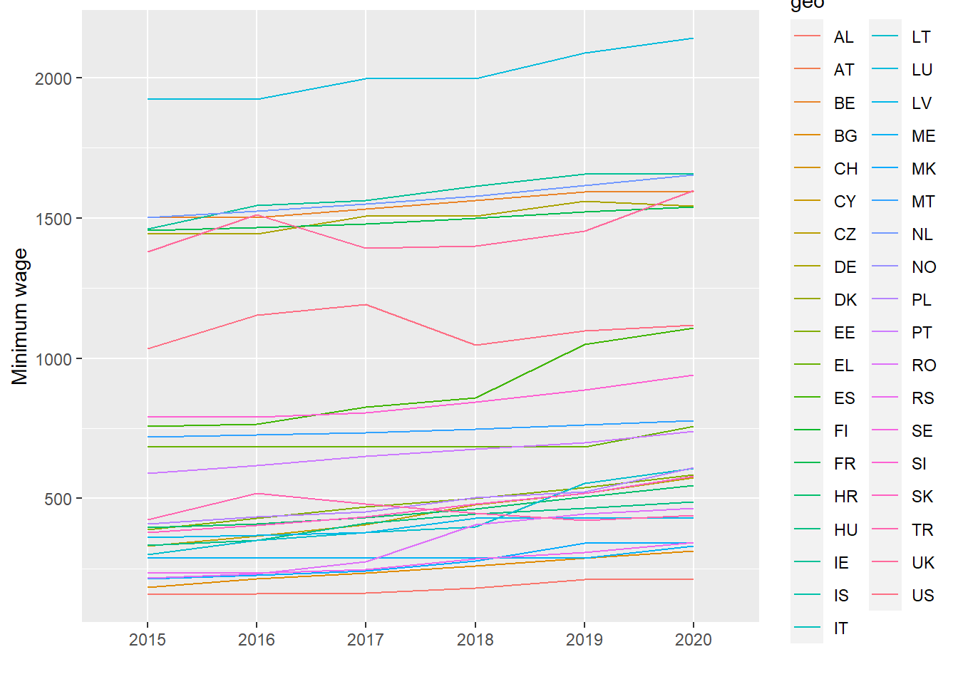
There has been a slight increase in the minimum wage in most European countries from 2015 to 2020. (This is probably because the varible is in euro which is not adjusted for the change in prices). We could adjust for change in prices, but then we have to download another dataset from the Eurostat-database which contains the price index for each country, and then adjust the minimum wage by the price index by adding them together.
21.4 Join the datasets together
Look at the datasets below. Which variables do they have in common (keys)?
head(unexp_reduced)# A tibble: 6 × 4
hhtyp geo time unexp_percent
<chr> <chr> <chr> <dbl>
1 A1F AL 2020 62.3
2 A1F AT 2020 24.7
3 A1F BE 2020 32.4
4 A1F BG 2020 78.7
5 A1F CH 2020 21.1
6 A1F CY 2020 47.2head(pop_reduced)# A tibble: 6 × 3
geo time n_people
<chr> <chr> <dbl>
1 AL 2020 2845955
2 AM 2020 2959694
3 AT 2020 8901064
4 AZ 2020 10067108
5 BE 2020 11522440
6 BG 2020 6951482head(minwage_reduced)# A tibble: 6 × 3
geo time minwage_eur
<chr> <chr> <dbl>
1 AL 2020 213.
2 AT 2020 NA
3 BE 2020 1594.
4 BG 2020 312.
5 CH 2020 NA
6 CY 2020 NA # geo and timedf <- unexp_reduced %>%
filter(hhtyp == "TOTAL") %>% # Only filter out the "TOTAL" from the hhtyp-variable, this gives us the financial insecurity for all household types.
left_join(pop_reduced, by = c("geo", "time")) %>% # join with the pop_reduced dataset.
left_join(minwage_reduced, by = c("geo", "time")) # join with the minwage_reduced dataset. Use the joined datasets to plot the relationship between minimum wage and financial insecurity in the European countries. - Colour them by country - Add a linear regression line - What do this plot tell us?
df %>%
  ggplot(aes(x = minwage_eur, y = unexp_percent)) +
  geom_point(aes(color = geo)) +
  geom_smooth(method = "lm")
`geom_smooth()` using formula = 'y ~ x'Warning: Removed 94 rows containing non-finite values (`stat_smooth()`).Warning: Removed 94 rows containing missing values (`geom_point()`).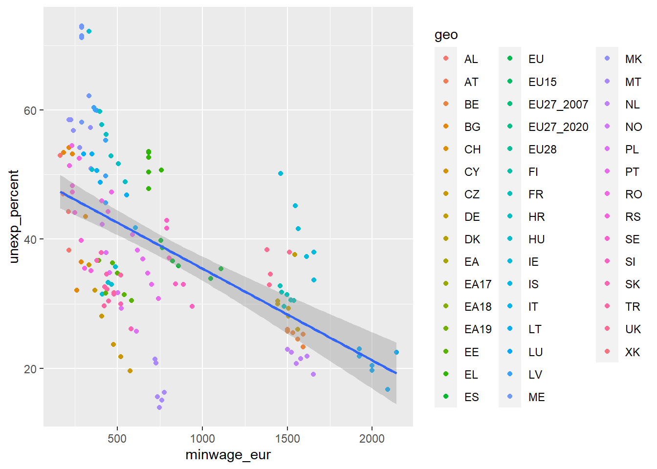
There is a negative bivariate correlation between financial insecurity and minimum wage. The lower the minimum wage, the higher the financial insecurity for European countries between 2015 and 2020.
21.5 Model
Make a linear model with unexp_percent as the dependent variable and minwage_eur, n_peopleand time as independent variables. Make time into a categorical variable (to construct a dummy variable in the regression).
model1 <- lm(unexp_percent ~ minwage_eur + n_people + factor(time),
              na.action = "na.exclude",
data = df)summary(model1) # Make a summary of the model.
Call:
lm(formula = unexp_percent ~ minwage_eur + n_people + factor(time),
    data = df, na.action = "na.exclude")

Residuals:
     Min       1Q   Median       3Q      Max
-25.3129  -7.0427  -0.6027   7.5435  27.2066

Coefficients:
                   Estimate Std. Error t value Pr(>|t|)
(Intercept)       5.412e+01  2.399e+00  22.558  < 2e-16 ***
minwage_eur      -1.311e-02  1.692e-03  -7.746 1.31e-12 ***
n_people         -5.463e-08  3.538e-08  -1.544   0.1247
factor(time)2016 -1.358e+00  2.940e+00  -0.462   0.6450
factor(time)2017 -3.544e+00  2.913e+00  -1.216   0.2257
factor(time)2018 -6.021e+00  2.914e+00  -2.066   0.0406 *
factor(time)2019 -7.439e+00  2.944e+00  -2.526   0.0126 *
factor(time)2020 -7.313e+00  2.947e+00  -2.481   0.0142 *
---
Signif. codes:  0 '***' 0.001 '**' 0.01 '*' 0.05 '.' 0.1 ' ' 1

Residual standard error: 10.6 on 150 degrees of freedom
  (94 observations deleted due to missingness)
Multiple R-squared:  0.3793,    Adjusted R-squared:  0.3503
F-statistic: 13.1 on 7 and 150 DF, p-value: 4.241e-13library(stargazer) # Open the stargazer-package.
Please cite as: Hlavac, Marek (2022). stargazer: Well-Formatted Regression and Summary Statistics Tables. R package version 5.2.3. https://CRAN.R-project.org/package=stargazer stargazer(model1, # Make a nice table of model1
type = "text") # Print the table in console
===============================================
                        Dependent variable:
                    ---------------------------
                           unexp_percent
-----------------------------------------------
minwage_eur                  -0.013***
                              (0.002)

n_people                     -0.00000
                             (0.00000)

factor(time)2016              -1.358
                              (2.940)

factor(time)2017              -3.544
                              (2.913)

factor(time)2018             -6.021**
                              (2.914)

factor(time)2019             -7.439**
                              (2.944)

factor(time)2020             -7.313**
                              (2.947)

Constant                     54.124***
                              (2.399)

-----------------------------------------------
Observations                    158
R2                             0.379
Adjusted R2                    0.350
Residual Std. Error      10.601 (df = 150)
F Statistic           13.095*** (df = 7; 150)
===============================================
Note:               *p<0.1; **p<0.05; ***p<0.01
21.5.1 Plot the effect of model1
Make a vector in which the minwage_eur-variable varies between the minimum value and the maximum value
minwage_eur_vektor = c(seq(min(df$minwage_eur, na.rm = TRUE),
                           max(df$minwage_eur, na.rm =TRUE),
                           by = 10)) # Let the variable vary in an interval of 10
n_people_vektor <- mean(df$n_people, na.rm = TRUE) # Make a vector with the average of n_people (population size) time_vektor <- "2017" # Make a vector with the with the year 2017Put all the vectors into one dataset. Name the variables minwage_eur, n_people and time. What type of constructed world is this?
snitt_data <- data.frame(minwage_eur = minwage_eur_vektor,
                         n_people = n_people_vektor,
                         time = time_vektor)
This is a world in which we have 193 countries (the number of rows in the dataset snitt_data). The year is 2017, all countries have 62.678.031 inhabitants, and the minimum wage is between 162,69 euro and 2082,69 euro.
Use the dataset snitt_data to predict the percentage with financial insecurity with the model you made.
pred_verdier <- predict(model1,
                        newdata = snitt_data,
                        se = TRUE, interval = "confidence")
Add the vectors which was made with predict() in the dataset snitt_data, so we have new columns.
snitt_data <- cbind(snitt_data, pred_verdier)What is the predicted percentage with financial insecurity for a country in 2017 with 62.678.031 inhabitants and minimum wage of 412.69 euro?
snitt_data %>%
  filter(minwage_eur == 412.69) %>%
  select(fit.fit)
fit.fit
26 41.64831# 42 percentWhat is the predicted percentage with financial insecurity for a country in 2017 with 62.678.031 inhabitants and minimum wage at the average of the minwage-vector?
snitt_data %>%
  filter(minwage_eur == mean(minwage_eur_vektor)) %>%
  select(fit.fit)
[1] fit.fit
<0 rows> (or 0-length row.names)# 32 percentWhat is the lower confidence interval of the predicted percentage with financial insecurity for a country in 2017 with 62.678.031 inhabitants and minimum wage at the maximum of the minwage-vector?
snitt_data %>%
  filter(minwage_eur == max(minwage_eur_vektor)) %>%
  select(fit.lwr)
fit.lwr
198 12.86872# 13 percentPlot the impact of minimum wage on financial insecurity.
snitt_data %>%
  ggplot(aes(x = minwage_eur, y = fit.fit)) +
  geom_line() +
  geom_ribbon(aes(ymin = fit.lwr,
                  ymax = fit.upr),
              alpha = .2) +
  labs(x = "Minimum wage", y = "Expected financial insecurity")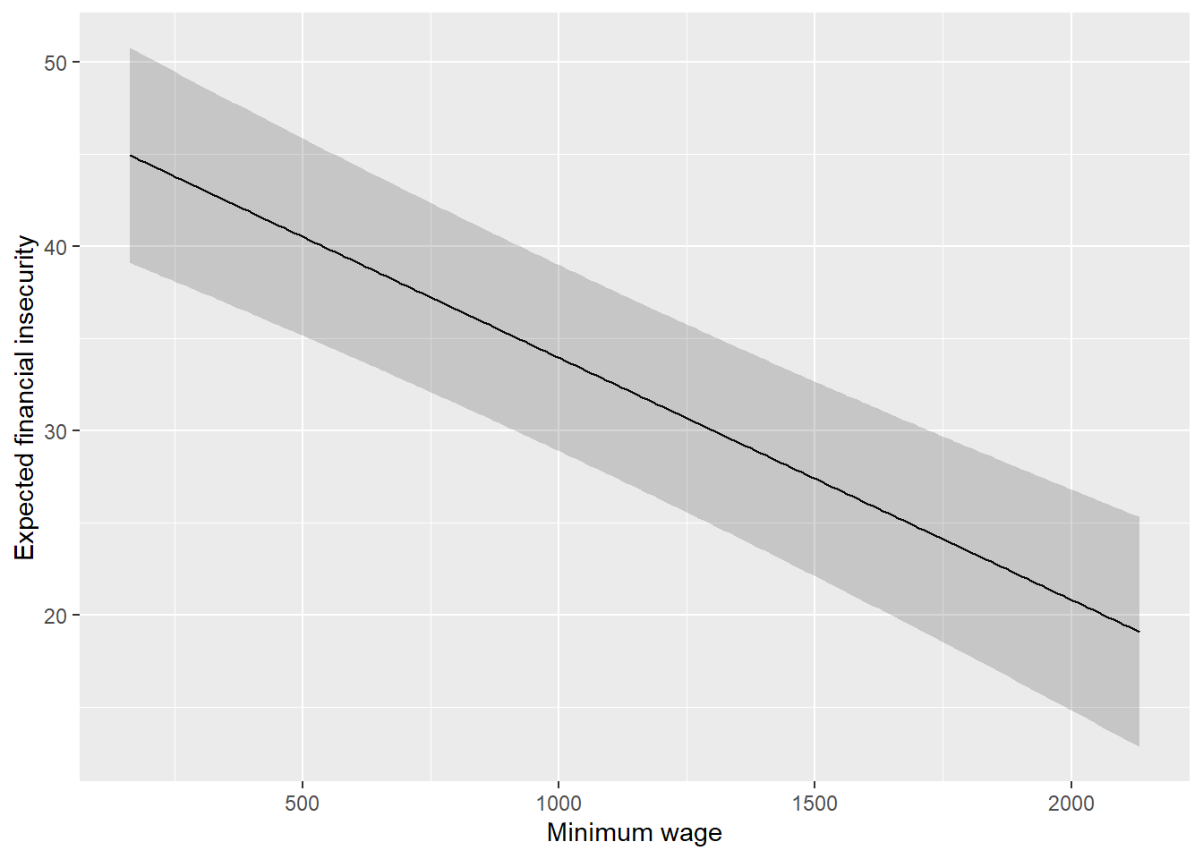
Concerning what we have done so far, do you think this is a good model to use to answer our research question (see the top of the script)? Is there something you would have done different?
Yes! For example:
Include more independent variables to avoid omitted variable bias.
Create an index for financial insecurity with more variables.
Adjust minimum wage for the increase in prices.
Include more years.
Check the conditions for OLS.
Get data for individuals’ financial insecurity on micro level and run a multivariate analysis.