library(tidyverse)

costofliving <- read_csv("../datafolder/costofliving.csv")

costofliving <- read_rds("../datafolder/costofliving.rds")

load("../datafolder/costofliving.rda")

load("../datafolder/costofliving.RData")

costofliving <- as_tibble(costofliving)10 How to import data
Most work will start with a stage of importing data. There are many ways getting data, for example from the databases, the web or API. For now, let’s look at how to import regular data stored in .csv, .RData, .rda or .rds.
First, recall that we store things in objects when working in R. So give your data a name, add an arrow <-, and then write a function to read in the data. The function you need depends on the format the data is stored in.
- data.csv :
read_csv - data.rds :
read_rds - data.RData :
load - data.rda :
load
End with the folder path and the name of the dataset in quotation marks, "".
Here, we’ll work with the dataset costofliving, a dataset that tracks the cost of living by cities in 2022, gathered from this website. On the website, the dataset is stored in .csv. I show here what the code would be if the data was stored in .rds, rda and .RData.
The functions are from the tidyverse package. Therefore, load this package in using library. I also transform the dataset to a tibble, which is the name of the type of dataframe used in the tidyverse.
10.1 The dataframe
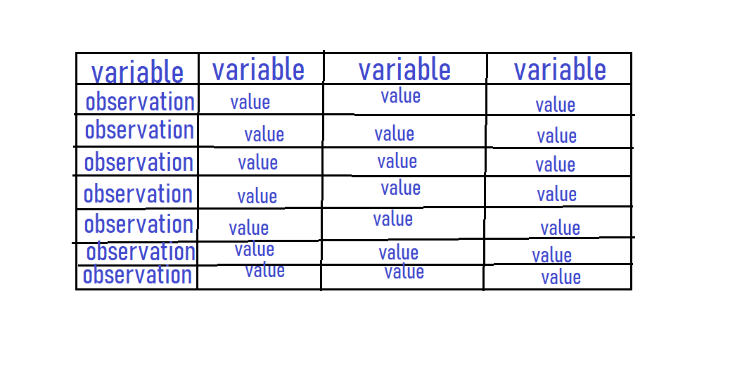
So what does the data look like when we’re doing quantitative analysis? Usually, we want the dataset to be in a dataframe. A dataframe has three components:
- Rows: Observations
- Columns: Variables
- Cells: Values
| Variable (e.g. number of inhabitants) | |
|---|---|
| Observation (e.g. Spain) | Value (e.g. 46.000.000) |
The observations are the entities we have in our dataset, for example countries, people, time period, or likewise. Variables are the properties of our entities, for example size or type. The values are the mix between these – the specific property that this specific entity has.
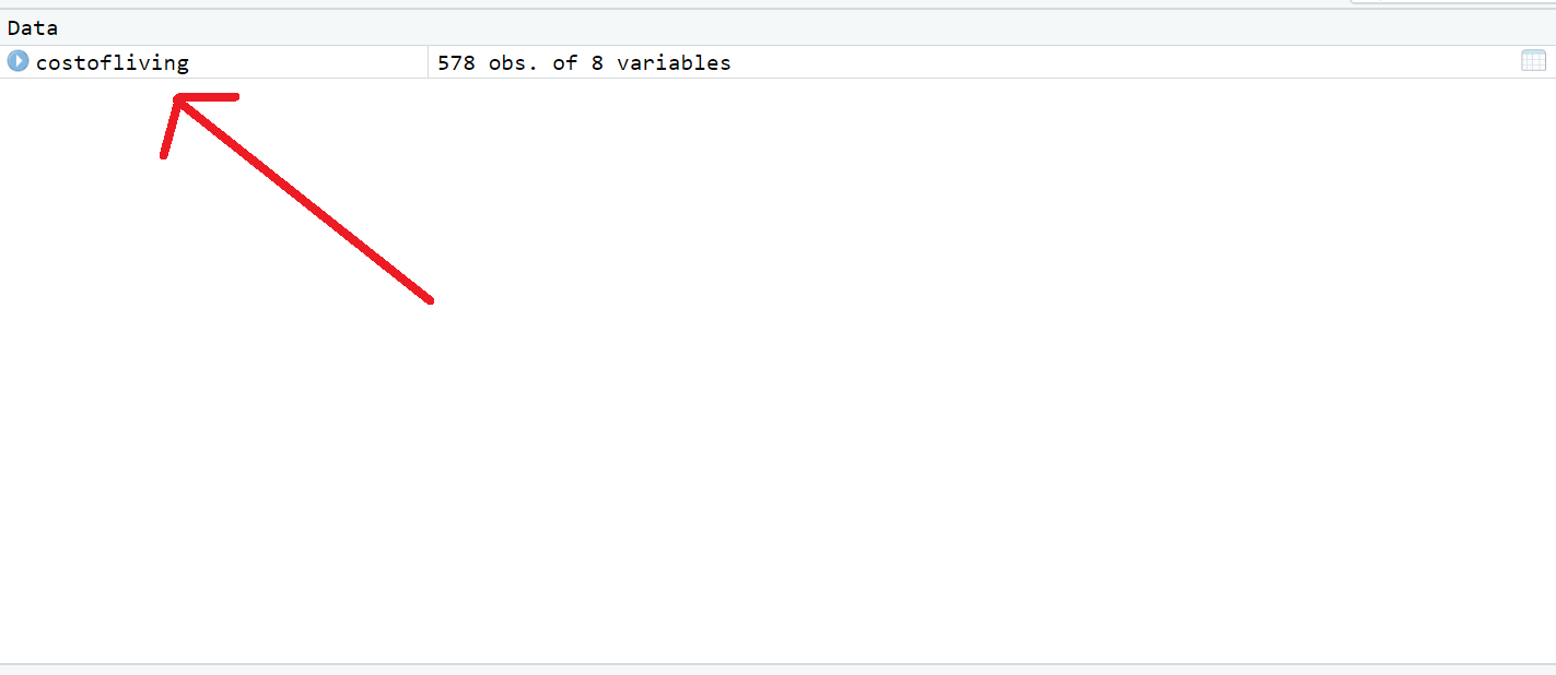
To see what our dataset looks like, you can click on the name of the dataset in the upper right corner of RStudio.
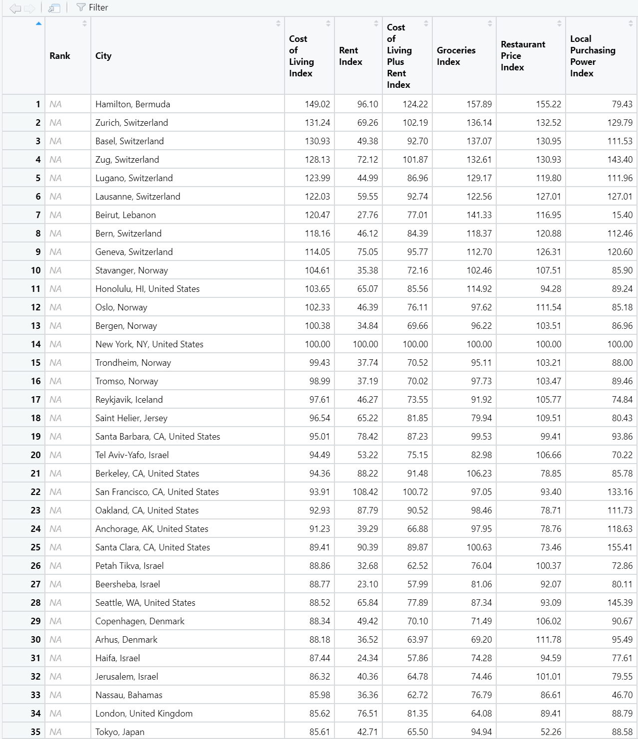
This dataset looks like below. The City variable denotes the observation – the city and the corresponding country. The other variables denote properties of these cities, cost of living, rent index and so on.
Another way of getting a look of the data in R is to use the function glimpse.
glimpse(costofliving)Rows: 578
Columns: 7
$ City <chr> "Hamilton, Bermuda", "Zurich, Switzerla…
$ Cost.of.Living.Index <dbl> NA, 131.24, NA, 128.13, 123.99, 122.03,…
$ Rent.Index <dbl> 96.10, 69.26, 49.38, 72.12, 44.99, 59.5…
$ Cost.of.Living.Plus.Rent.Index <dbl> 124.22, 102.19, NA, 101.87, 86.96, 92.7…
$ Groceries.Index <dbl> 157.89, 136.14, 137.07, 132.61, 129.17,…
$ Restaurant.Price.Index <dbl> 155.22, 132.52, 130.95, NA, 119.80, 127…
$ Local.Purchasing.Power.Index <dbl> 79.43, 129.79, 111.53, 143.40, 111.96, …10.2 About the dataset
These indices are relative to New York City (NYC). Which means that for New York City, each index should be 100(%). If another city has, for example, rent index of 120, it means that on an average in that city rents are 20% more expensive than in New York City. If a city has rent index of 70, that means on average rent in that city is 30% less expensive than in New York City.
Cost of Living Index (Excl. Rent) is a relative indicator of consumer goods prices, including groceries, restaurants, transportation and utilities. Cost of Living Index does not include accommodation expenses such as rent or mortgage. If a city has a Cost of Living Index of 120, it means Numbeo has estimated it is 20% more expensive than New York (excluding rent).
Rent Index is an estimation of prices of renting apartments in the city compared to New York City. If Rent index is 80, Numbeo has estimated that price of rents in that city is on average 20% less than the price in New York.
Groceries Index is an estimation of grocery prices in the city compared to New York City. To calculate this section, Numbeo uses weights of items in the “Markets” section for each city.
Restaurants Index is a comparison of prices of meals and drinks in restaurants and bars compared to NYC.
Cost of Living Plus Rent Index is an estimation of consumer goods prices including rent comparing to New York City.
Local Purchasing Power shows relative purchasing power in buying goods and services in a given city for the average net salary in that city. If domestic purchasing power is 40, this means that the inhabitants of that city with an average salary can afford to buy on an average 60% less goods and services than New York City residents with an average salary.