library(rvest)
library(stringr)

song_page <- read_html("https://www.westsidestory.com/lyrics") # Read the html page

songs <- song_page %>%
  html_nodes("h2") %>% # Extract all html-nodes with the tag <h2>
  html_elements("a") %>% # Extract from this node all html-tags with <a>
  html_attr("href") %>% # And from these, the text belonging to the link reference <href>
  str_c("https://www.westsidestory.com", .)  # Paste together the previous webpage string with these

headline <- str_remove_all(songs, "https://www.westsidestory.com/") # Extracting the name of the songs32 Text tokenization
To make text possible to process by a computer, we need to break the text down into units of information. This process is called tokenization. Some teaching materials on text analysis treat tokenization as a part of text preprocessing, and in truth, the two are rather overlapping. For example, it is not unusual to remove stopwords after having tokenized the text. Another part of preprocessing is stemming, which means taking the root (base) of a word. We’ll come back to this, and how to plot text, but first we’ll see how to tokenize.
As an example in this lecture, we’ll use songs from the musical West Side Story. As a bit of repetition, we’ll do some webscraping to fetch the song lyrics from a webpage on the internet.
for(i in 1:length(songs)) { # For all the links to the different songs...

  download.file(songs[[i]], # Download one html-file after another into the folder specified in destfile
                destfile = str_c("../datafolder/ws_songs/", headline[i], ".html"))
}
songfiles <- list.files("../datafolder/ws_songs/") %>%
str_c("../datafolder/ws_songs/", .) # Listing up the html-files in the folder
songname <- list() # Make an empty list for the songnames
ws_lyrics <- list() # Make an empty list for the lyrics
for(i in 1:length(songfiles)){ # For each file in the folder as listed
songname[[i]] <- songfiles[i] %>%
str_remove("../datafolder/ws_songs/") %>% # Remove the beginning of the file string
str_remove("\\.html") # Remove the end - leaving us with just the name of the song
lyric <- read_html(songfiles[i]) # Read the html-page
lyric <- lyric %>%
html_node("p") %>% # Extract all nodes with the tag <p>
html_text2() # Fetch the text from these tags
ws_lyrics[[i]] <- lyric # Add the lyrics to the empty list
}
ws_lyrics <- str_replace_all(ws_lyrics, "\n", " ") # Replacing double lineshift with space to make the next code work
ws_lyrics <- str_remove_all(ws_lyrics, "\\b[A-Z]{2,}\\b") # Remove all sequences of big letters followed by lineshift, as they are names of who's singing
westside <- as_tibble(list(songname = unlist(songname), # Put the songnames into a column in a tibble
lyrics = unlist(ws_lyrics))) # Put the lyrics into a column in a tibble
glimpse(westside)Rows: 14
Columns: 2
$ songname <chr> "a-boy-like-thati-have-a-love", "america", "cool", "finale", …
$ lyrics <chr> " A boy like that who'd kill your brother, Forget that boy an…32.1 How to tokenize text
When we tokenize, we split the text up into units. Most often, these units are words1. Tokenizing the units into words means that the order of the words disappear. Studies have shown that often, it is not the order of the words but the choice of words that give us the most information on what the text is about. However, if we speculate that the order of the words might matter, we can also split the text into two and two words, three and three words, or whole sentences. When we tokenize into one word, we refer to these units and unigrams. Two words are bigrams, three words are trigrams and so on. Together, they are called n-grams.
To tokenize our group of texts (sometimes referred to as a corpus of text), we’ll be using the package tidytext.
library(tidytext)This package assumes that your data is in a dataframe. So if it’s in a list, put it into a dataframe using for example do.call(rbind, list) or enframe. Once that is done, use the unnest_tokens function to tokenize the text. As arguments, add as input the name of the old column with the text, as output the name of the new column you are creating, and as token we specify “words” to get unigrams.
westside_tokens <- westside %>%
  unnest_tokens(input = lyrics, # Which variable to get the text from
                output = word, # What the new variable should be called
                token = "words") # What kind of tokens we want to split the text into

westside_tokens
# A tibble: 2,624 × 2
songname word
<chr> <chr>
1 a-boy-like-thati-have-a-love a
2 a-boy-like-thati-have-a-love boy
3 a-boy-like-thati-have-a-love like
4 a-boy-like-thati-have-a-love that
5 a-boy-like-thati-have-a-love who'd
6 a-boy-like-thati-have-a-love kill
7 a-boy-like-thati-have-a-love your
8 a-boy-like-thati-have-a-love brother
9 a-boy-like-thati-have-a-love forget
10 a-boy-like-thati-have-a-love that
# ℹ 2,614 more rowsHad we wanted bigrams, we could specify token = "ngrams" and n = 2.
westside %>%
  unnest_tokens(input = lyrics,
                output = word,
                token = "ngrams",
                n = 2)
# A tibble: 2,610 × 2
songname word
<chr> <chr>
1 a-boy-like-thati-have-a-love a boy
2 a-boy-like-thati-have-a-love boy like
3 a-boy-like-thati-have-a-love like that
4 a-boy-like-thati-have-a-love that who'd
5 a-boy-like-thati-have-a-love who'd kill
6 a-boy-like-thati-have-a-love kill your
7 a-boy-like-thati-have-a-love your brother
8 a-boy-like-thati-have-a-love brother forget
9 a-boy-like-thati-have-a-love forget that
10 a-boy-like-thati-have-a-love that boy
# ℹ 2,600 more rowsOr we can tokenize into sentences.
westside %>%
  unnest_tokens(input = lyrics,
                output = word,
                token = "sentences")
# A tibble: 275 × 2
songname word
<chr> <chr>
1 a-boy-like-thati-have-a-love a boy like that who'd kill your brother, forget…
2 a-boy-like-thati-have-a-love stick to your own kind!
3 a-boy-like-thati-have-a-love a boy like that will give you sorrow.
4 a-boy-like-thati-have-a-love you'll meet another boy tomorrow, one of your o…
5 a-boy-like-thati-have-a-love stick to your own kind!
6 a-boy-like-thati-have-a-love a boy who kills cannot love, a boy who kills ha…
7 a-boy-like-thati-have-a-love and he's the boy who gets your love and gets yo…
8 a-boy-like-thati-have-a-love very smart, maria, very smart!
9 a-boy-like-thati-have-a-love a boy like that wants one thing only, and when …
10 a-boy-like-thati-have-a-love he'll murder your love; he murdered mine.
# ℹ 265 more rows32.2 Stopword removal with tokenized text
If we sort by songname and word and count the occurrences of words within each song, the variable n shows the number of words for each song from highest to lowest using sort = TRUE. Here, we see that stopwords such as “a”, “i” and “is” are occurring rather frequently.
westside_tokens %>%
  count(songname, word, sort = TRUE) # Counting the number of words per songsame and sorting from highest to lowest
# A tibble: 1,224 × 3
songname word n
<chr> <chr> <int>
1 gee-officer-krupke a 32
2 maria maria 23
3 i-feel-pretty pretty 19
4 tonight-quintet tonight 19
5 a-boy-like-thati-have-a-love i 17
6 america in 17
7 america america 16
8 gee-officer-krupke is 16
9 jet-song you're 16
10 i-feel-pretty and 15
# ℹ 1,214 more rowsTo remove the stopwords, we can use anti_join. This is an alternative to going back to the character vector in the list and work with regex. When we have the data stored as words in a column in a dataframe, we can join against another similar dataframe and remove the cells that have the same word. The tidytext package has an inbuilt dataframe called stop_words containing stopwords that we might want to remove. Notice that the column in the stop_words dataframe that we want to anti_join against is called word, which means that to make things easier for ourselves, the column in our dataframe should also be called word.
tidytext::stop_words # A dataframe with stopwords within the tidytext package# A tibble: 1,149 × 2
word lexicon
<chr> <chr>
1 a SMART
2 a's SMART
3 able SMART
4 about SMART
5 above SMART
6 according SMART
7 accordingly SMART
8 across SMART
9 actually SMART
10 after SMART
# ℹ 1,139 more rowswestside_tokens <- westside_tokens %>%
anti_join(stop_words, by = "word") # Joining against the stopwords dataframe to get rid of cells with stopwords
westside_tokens %>%
count(songname, word, sort = TRUE)# A tibble: 568 × 3
songname word n
<chr> <chr> <int>
1 maria maria 23
2 i-feel-pretty pretty 19
3 tonight-quintet tonight 19
4 america america 16
5 tonight-duet tonight 13
6 i-feel-pretty feel 12
7 cool boy 11
8 a-boy-like-thati-have-a-love love 10
9 gee-officer-krupke krupke 9
10 a-boy-like-thati-have-a-love boy 8
# ℹ 558 more rowsThat looks better! If you have bigrams and want to remove stopwords using this method, have a look at chapter 4 in Tidytext.
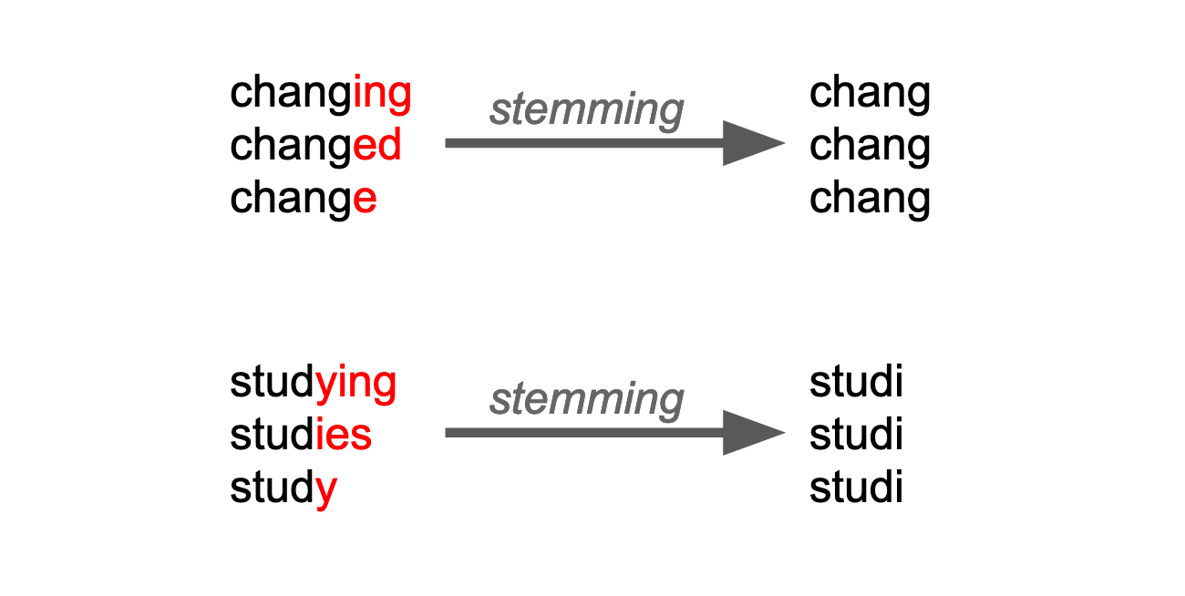
32.3 Stemming the word
Consider the words “have”, “having” and “had”. Would you say that they are more or less different than “have” and “run”? Inflections of words usually do more to the noise in our dataset than give useful information. Because once the word is spelled differently, computer interprets the words as completely distinct words. That is why we often choose to stem. In the word “wait”, for example, stemming involves recuding the word to “wait” for all its different inflections:
- wait (infinitive)
- wait (imperative)
- waits (present, 3rd person, singular)
- wait (present, other persons and/or plural)
- waited (simple past)
- waited (past participle)
- waiting (progressive)
So stemming means taking the stem of the word, also called the root or the base. This goes for verbs and nouns alike, and it might involve chopping off parts of the words such as affixes and suffixes2.
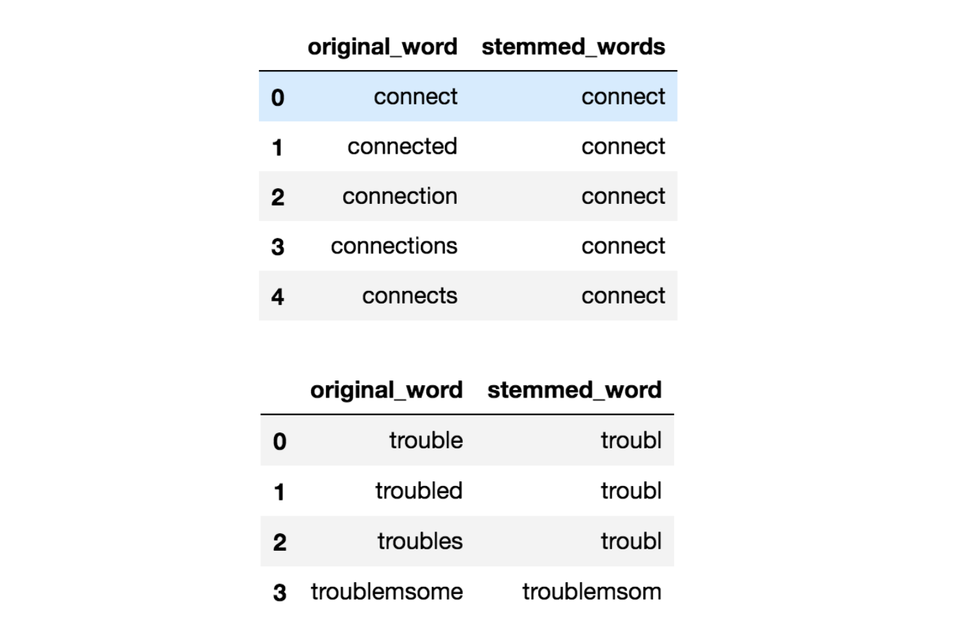
To stem tokens in R, load a wordstemming package such as SnowballC and use the function wordStem on the variable with the tokens.
library(SnowballC)

westside_tokens <- westside_tokens %>%
  mutate(stem = wordStem(word))
32.4 Plotting tokenized text
One way of extracting insight from text is to tokenize it and then plot it.
plot_df <- westside_tokens %>% # Make a new dataframe to plot
  count(songname, stem) %>% # Counting the number of words per songname
  group_by(songname) %>% # Grouping by songname and...
  slice_max(n, n = 5) %>% # Taking out the five top most used words per songname
  ungroup() # Ungrouping to get the dataframe back to normal

plot_df %>%
  ggplot(aes(n, fct_reorder(stem, n), # Placing number of occurences (n) on the x-axis and word on the y-axis
             fill = songname)) + # Adding colors to the bars after the songname
  geom_bar(stat = "identity") + # Making a barplot where the y-axis is the measure (stat = "identity")
  facet_wrap(~ songname, ncol = 4, scales = "free") + # Making one small plot per songname, arranging them in three columns and let the y-axis vary independent of the other plots
  labs(x = "", y = "") + # Removing all labels on x- and y-axis
  theme_bw() + # Make the background white
  theme(legend.position = "none") # Removing the legend for what colors mean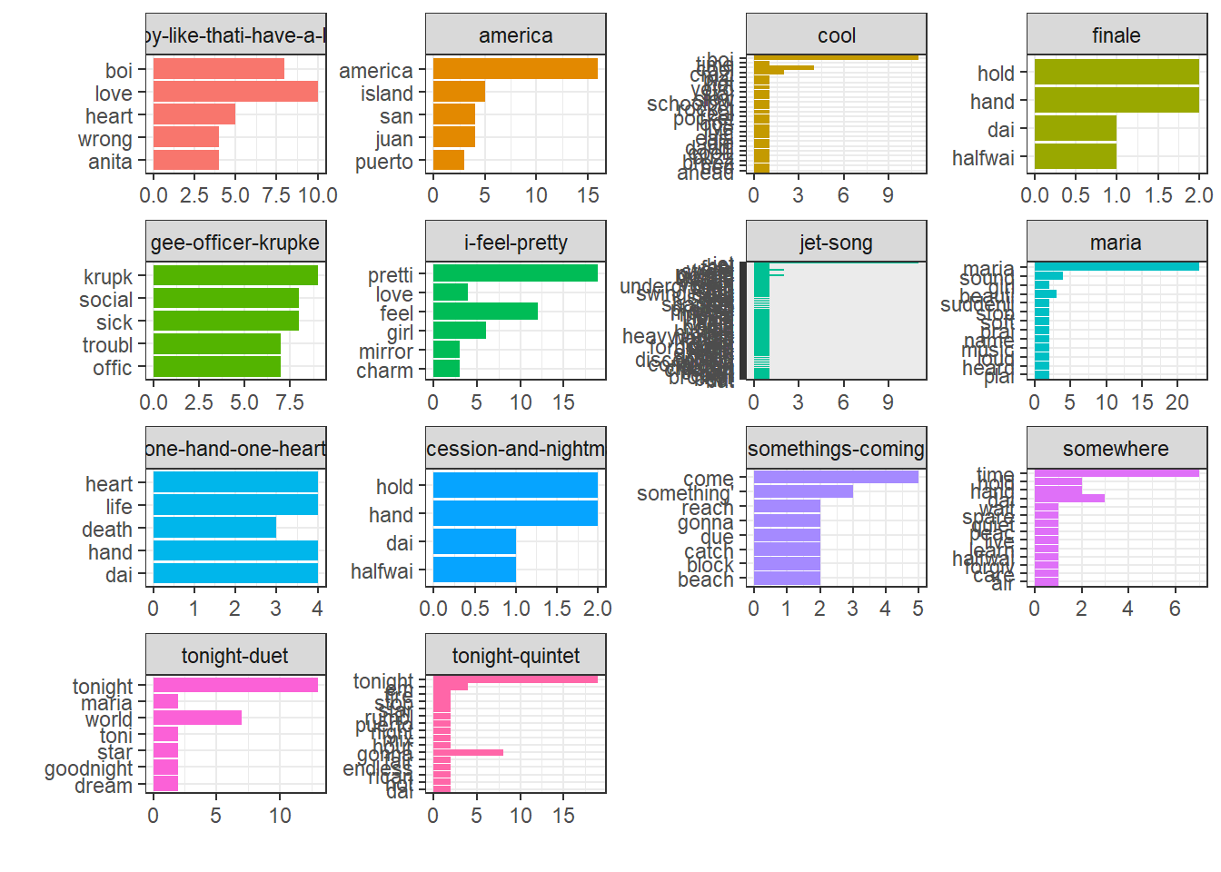
Or, we can make a wordcloud. There are many packages available to make wordclouds, in this case, I use the wordcloud package.
library(wordcloud) # Loading one package that we can use to make wordclouds

wordcloud_df <- westside_tokens %>%
  count(songname, stem) # Counting the number of words per songname

wordcloud_df %>%
  with(wordcloud(stem, n, # Making a wordcloud with the words weighed by how frequent they are
                 max.words = 100, # Plotting maximum 100 words to not make the plot too big
                 colors = brewer.pal(8, "Dark2")[factor(westside_tokens$songname)])) # Coloring the words after which songname they come from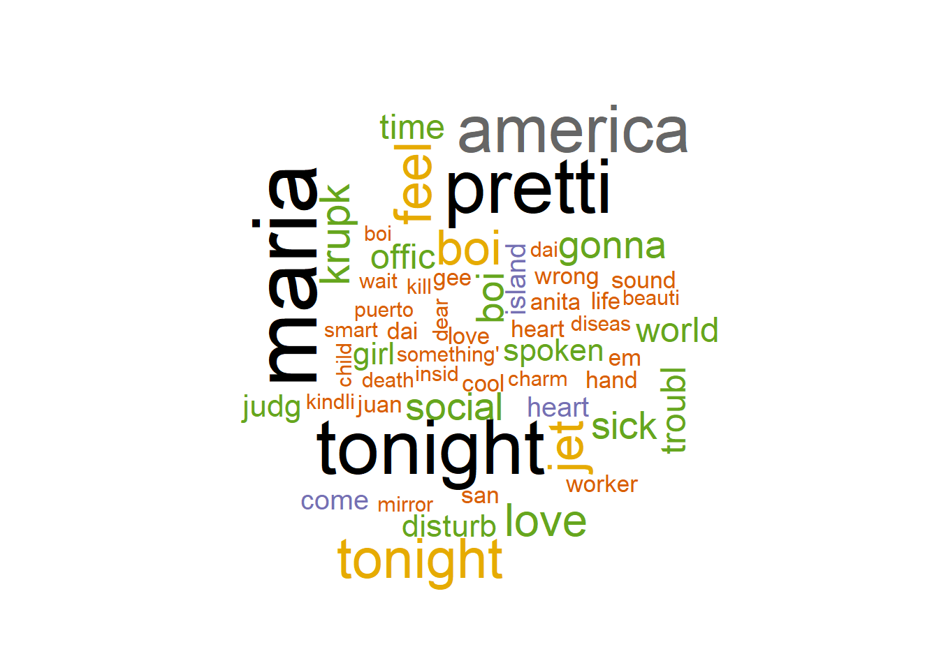
They can also be syllables or groups or words or many other things↩︎
A more nuanced way of recuing a word to its root is to use lemmatization. Here, you also take into account the context in which the word appears. It is a more complex method and often not necessary, but it can be fruitful in some analyses.↩︎