20 Tasks: Descriptive statistics
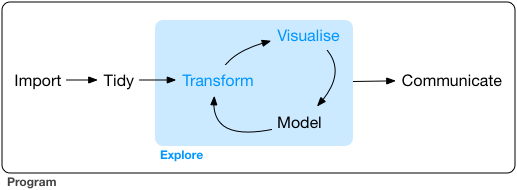
This worksheet is centered around the workflow in the picture below. Using the example research question below, we are going to see how one can go from having data and a question, to perhaps finding some answers.
Research question: Is there a positive correlation between minimum wage and your experienced financial security, in EU-countries from 2015 until 2020?
Task: Fill in the blank spaces (___) in the code.
20.1 Importing data
First, we need to install and library in the necessary packages.
install.___("eurostat") # Installing the package "eurostat"Eurostat is the statistical office of the European Union. They have made their own R-package which we can use to gather data directly from their database with the use of code. For a full overview of their database, see this link.
___(eurostat)
___(tidyverse)
We use the function get_eurostat() to upload data from the Eurostat package to R. Make sure you are connected to wifi when you run the code.
Fetch the datasets shown below and give the datasets we upload the following names: unexp, pop, and minwage.
___ <- get_eurostat("ilc_mdes04") # Percentage of population with inability to face unexpected financial expenses
___ <- get_eurostat("demo_pjan") # Population on 1 January by age and sex
___ <- get_eurostat("earn_mw_cur") # Monthly minimum wages - bi-annual data
20.2 Tidy and transform
20.2.1 1. Get an overview of the data
head(unexp) # Printing the six first rows of the dataset unexp.
glimpse(unexp) # Have a look at the type of variables, and the number of rows and columns in the dataset unexp.___(___) # Printing the six first rows of the dataset pop.
___(___) # Have a look at the type of variables, and the number of rows and columns in the dataset pop.___(___) # Printing the six first rows of the dataset minwage
___(___) # Have a look at the type of variables, and the number of rows and columns in the dataset minwage.names(___) # Put one of the datasets into this function, what does the function tell us about the dataset?
# We see the variable names (column names) in the datasetnrow(___) # Put another dataset into this function, what does the function tell us about the dataset?
# We see the number of observations (number of rows) in the dataset. 20.2.2 2. Missing values
unexp %>%
  ___.cases() # Print a table that shows us all units with missing values on at least one variable.

minwage %>%
  ___(values) %>% # Get the variable "values" from the dataset.
  is.na() %>%
  ___() # Count the number of units which are missing on the variable "values".
20.2.3 3. Are the variables useful?
The time-variable
table(unexp$time) # Print the values of the variable "time" from the dataset "unexp".- What does this variable tell us? Is it useful?
- Is it important for us to know that the data is for the 1st of January each year, or only that its valid for that year?
- Do we need data for all years? (see the research question at the top of the script)
unexp_reduced <- unexp %>% # change the variable "time" with the function ifelse() so it only contains the year, and not the date.
  mutate(time = ifelse(time == "___", "2015",
                       ifelse(time == "___", "2016",
                              ifelse(time == "___", "2017",
                                     ifelse(time == "___", "2018",
                                            ifelse(time == "___", "2019",
                                                   ifelse(time == "___", "2020",
                                                          time))))))) %>%
filter(time %in% c("___", "___", "___", "___", "___", "___")) # Get the rows with the years 2015, 2016, 2017, 2018, 2019 and 2020. table(___$time) # Check if your code is correct. Remember that we have now made a new dataset with a new name. ___(___$___) # Check if the dataset "pop" has it's time-variable coded the same way as in the dataset unexp. # A more efficient approach to getting only the year from the "date" variable
pop_reduced <- pop %>%
___(time = substr(time, 1, 4)) # Make a new variable "time" in the dataset "pop" with only year, not datepop_reduced <- pop_reduced %>%
filter(___ %in% c("2015", "2016", "2017", "2018", "2019", "2020")) # Get only the years we needThe minwage-dataset is different. It is biannual, which means that it’s for every other year.
table(minwage$time) Since the other datasets we have are for years, this dataset also need to be in years for us to compare them. Therefore we get the rows with minimum wage for the 1st of January.
# Make sure the following code is in the right order:
  mutate(time = substr(time, 1, 4)) %>%

  filter(time %in% c("2015", "2016", "2017", "2018", "2019", "2020"))

minwage_reduced <- minwage %>%

  filter(!time %in% c("2020-07-01", "2019-07-01", "2018-07-01", "2017-07-01", "2016-07-01", "2015-07-01")) %>%

  mutate(time = as.character(time)) %>%
The value-variable
class(unexp_reduced$___) # Find the class of the variable "values" in the unexp-dataset. Comment what the class is. ___(unexp_reduced$values, na.rm = TRUE) # Find the maximum value of the variable "values" in the dataset unexp.
___(unexp_reduced$values, na.rm = TRUE) # Find the minimum value of the variable "values" in the dataset unexp.What does this variable tell us?
head(unexp_reduced)
table(unexp_reduced$unit)
Run the code above and look at the variable “unit”. It has the value “PC”. This indicates that the variable “values” is given in percentage. So the “values” show the percentage in each EU-country (“geo”) who says that they could not manage a sudden financial cost (according to household type (“hhtyp”) and income group (“incgrp”)).
Is “values” a useful name for the variable?
unexp_reduced <- unexp_reduced %>%
  ___(unexp_percent = values) # Change the name of the variable from "values" to "unexp_percent".
Check if the datasets pop and minwage also have variables called “values”.
___(pop_reduced) # What type of value do you think the "values"-variable is given in? Comment below.
table(___$unit)___(minwage_reduced)
table(___$currency)Change the name of these variables as well.
pop_reduced <- pop_reduced %>%
  rename(n_people = ___)
minwage_reduced <- ___ %>%
rename(minwage_eur = values) 20.2.4 4. Are the observations useful?
What are the units in our research question? Which variable differentiate between the units in the dataset unexp? Comment below.
glimpse(unexp_reduced)
#
#
Which values are in the hhtyp-variable (household type)?
___(unexp_reduced$hhtyp)Which values are in the incgrp-variable (income group)?
___(unexp_reduced$incgrp)Get only the row with the value “TOTAL” from the incgrp-variable.
unexp_reduced <- unexp_reduced %>%
  filter(incgrp == "___")
Get from the hhtyp-variable only the rows with the values “A1F”, “A1M”, “A2” and “TOTAL”.
unexp_reduced <- unexp_reduced %>%
  ___(hhtyp %in% c("A1F", "A1M", "A2", "TOTAL"))
Now the variables “incgrp” and “unit” have the same values, and therefore does not give us more useful information. Remove the variables “incgrp” and “unit” from the dataset.
unexp_reduced <- unexp_reduced %>%
  select(hhtyp, geo, ___, ___)
We tidy the pop-dataset and the minwage-dataset in the same way. Fill in the code below so it’s correct.
pop_reduced <- pop_reduced %>%
  filter(age == "TOTAL") %>%
  filter(sex == "T") %>%
  ___(geo, time, n_people)
minwage_reduced <- minwage_reduced %>%
___(___ == "EUR") %>%
select(-(currency)) # Minus with select() removes the variables20.2.5 5. Descriptive statistics
Find the average percentage who says that they could manage a sudden financial cost.
___(unexp_reduced$unexp_percent, na.rm = TRUE) Change the variable n_people (population size) to log.
___(pop_reduced$n_people) Find the average percentage who says they could not manage a sudden financial cost, grouped by year and country
unexp_reduced %>%
  group_by(___, ___) %>%
  summarise(unexp_pc_mean = mean(___))
20.3 Visualize
Make a boxsplot with unexp_percent (percentage with financial insecurity) on the x-axis. geo (country) on the y-axis and colour by hhtyp (household type). What does this plot tell us?
unexp_reduced %>%
  ___(aes(x = unexp_percent, ___ = geo, color = hhtyp)) +
  geom_boxplot()
Filter out only the countries FR (France), DE (Germany), ES (Spain), BE (Belgium), NO (Norway), SE (Sweden) and DK (Denmark), then plot again. Recode the values on the hhtyp to something that is more understandable.
unexp_reduced %>%

  geom_boxplot()

ggplot(aes(x = unexp_percent, y = geo, color = hhtyp)) +

  filter(geo %in% c("FR", "DE", "ES", "BE", "NO", "SE", "DK")) %>%

  mutate(hhtyp = ifelse(hhtyp == "A1F", "Single women",
                        ifelse(hhtyp == "A1M", "Single men",
                               ifelse(hhtyp == "A2", "Two adults", hhtyp)))) %>%
Which country has the highest percentage who reports financial insecurity?
Which country has the lowest percentage who reports financial insecurity?
Which type of household has the highest percentage who reports financial insecurity?
What is the approximate median of the percentage who reports financial insecurity among households with two adults in Germany?
Plot the minimum wage for the European countries over time with a line diagram. Colour the dots by country.
minwage_reduced %>%
  ggplot(aes(x = time, y = minwage_eur, group = geo, ___ = geo)) +
  ___() +
  labs(x = "", y = "Minimum wage")
There has been a slight increase in the minimum wage in most European countries from 2015 to 2020. (This is probably because the varible is in euro which is not adjusted for the change in prices). We could adjust for change in prices, but then we have to download another dataset from the Eurostat-database which contains the price index for each country, and then adjust the minimum wage by the price index by adding them together.
20.4 Join the datasets together
Look at the datasets below. Which variables do they have in common (keys)?
head(unexp_reduced)
head(pop_reduced)
head(minwage_reduced)
# ___ and ___
df <- unexp_reduced %>%
filter(hhtyp == "___") %>% # Only filter out the "TOTAL" from the hhtyp-variable, this gives us the financial insecurity for all household types.
left_join(pop_reduced, by = c("___", "___")) %>% # join with the pop_reduced dataset.
left_join(minwage_reduced, by = c("___", "___")) # join with the minwage_reduced dataset. Use the joined datasets to plot the relationship between minimum wage and financial insecurity in the European countries. - Colour them by country - Add a linear regression line - What do this plot tell us?
df %>%
  ggplot(___(x = minwage_eur, y = unexp_percent)) +
  geom_point(aes(color = ___)) +
  geom_smooth(___ = "lm")
20.5 Model
Make a linear model with unexp_percent as the dependent variable and minwage_eur, n_peopleand time as independent variables. Make time into a categorical variable (to construct a dummy variable in the regression).
model1 <- lm(___ ~ ___ + ___ + factor(___),
              na.action = "na.exclude",
data = ___)summary(model1) # Make a summary of the model. ___(stargazer) # Open the stargazer-package.
stargazer(___, # Make a nice table of model1
type = "text") # Print the table in console20.5.1 Plot the effect of model1
Make a vector in which the minwage_eur-variable varies between the minimum value and the maximum value
minwage_eur_vektor = c(seq(___(df$minwage_eur, na.rm = TRUE),
                           ___(df$minwage_eur, na.rm =TRUE),
                           by = ___)) # Let the variable vary in an interval of 10
n_people_vektor <- mean(df$n_people, na.rm = TRUE) # Make a vector with the average of n_people (population size) time_vektor <- "___" # Make a vector with the with the year 2017Put all the vectors into one dataset. Name the variables minwage_eur, n_people and time. What type of constructed world is this?
snitt_data <- ___(minwage_eur = ___,
                         n_people = ___,
                         time = ___)
This is a world in which we have 193 countries (the number of rows in the dataset snitt_data). The year is 2017, all countries have 62.678.031 inhabitants, and the minimum wage is between 162,69 euro and 2082,69 euro.
Use the dataset snitt_data to predict the percentage with financial insecurity with the model you made.
pred_verdier <- ___(modell1,
                    newdata = ___,
                    se = TRUE, interval = "confidence")
Add the vectors which was made with predict() in the dataset snitt_data, so we have new columns.
snitt_data <- cbind(___, ___)What is the predicted percentage with financial insecurity for a country in 2017 with 62.678.031 inhabitants and minimum wage of 412.69 euro?
snitt_data %>%
  filter(minwage_eur == ___) %>%
  select(fit.fit)
What is the predicted percentage with financial insecurity for a country in 2017 with 62.678.031 inhabitants and minimum wage at the average of the minwage-vector?
snitt_data %>%
  filter(___ == ___(minwage_eur_vektor)) %>%
  select(fit.fit)
What is the lower confidence interval of the predicted percentage with financial insecurity for a country in 2017 with 62.678.031 inhabitants and minimum wage at the maximum of the minwage-vector?
snitt_data %>%
  filter(minwage_eur == max(___)) %>%
  select(___)
Plot the impact of minimum wage on financial insecurity. Order the lines correctly.
  geom_line() +

  labs(x = "Minimum wage", y = "Expected financial insecurity")

ggplot(aes(x = minwage_eur, y = fit.fit)) +

  geom_ribbon(aes(ymin = fit.lwr,
                  ymax = fit.upr),
              alpha = .2) +
Concerning what we have done so far, do you think this is a good model to use to answer our research question (see the top of the script)? Is there something you would have done different?