26 API
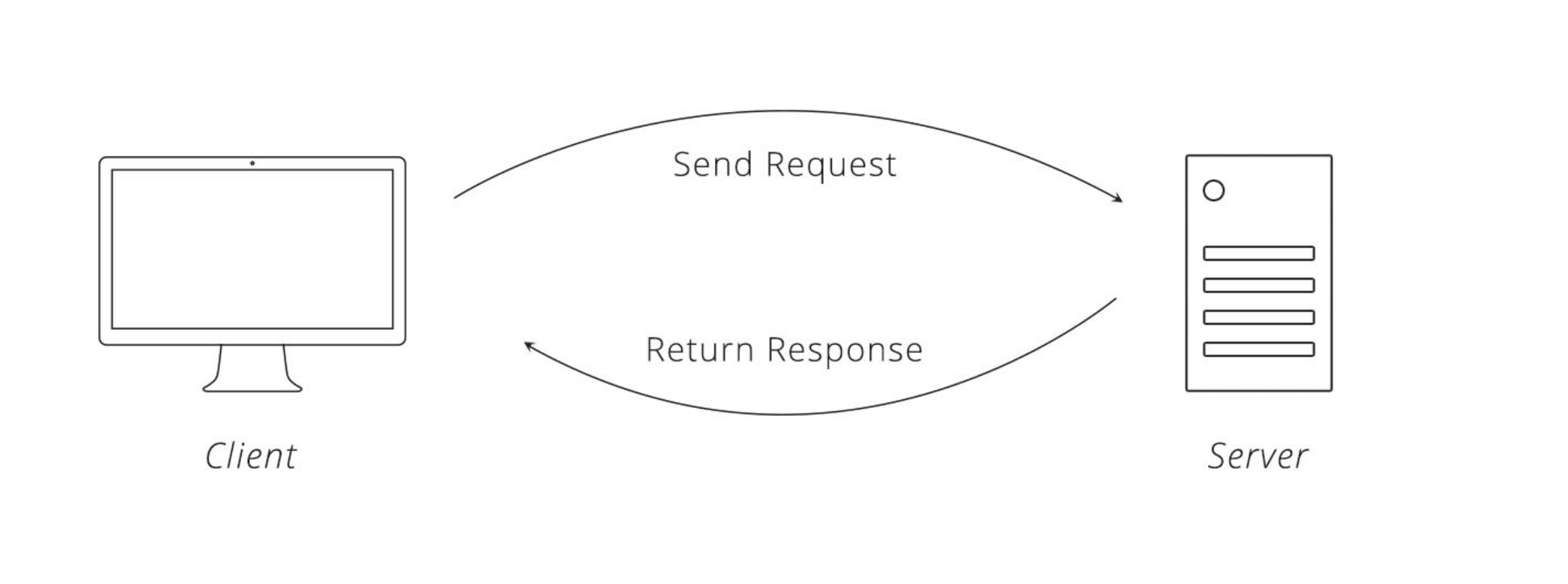
Have you ever talked to somebody about data collection and then gotten the question “do they have an API?”. For somebody who has never used APIs before, the concept can seem rather foreign, but it is extremely useful to know what APIs are and how to use them. API stands for Application Programming Interface, and basically, it is a way for the computer to handle contents on a webpage so that the computer can receive and deliver data easily. In other words, APIs are built for data transfer. For us, APIs improve upon previous ways of gathering data:
- Sending a mail and asking for some flat files (e.g.
.csv), often time-consuming and not always feasible. - Applying for access to others’ databases, which is often quite dubious.
- Webscraping content, meaning writing long scripts and adding pressure to the client’s server .
To be fair, APIs are about more than gathering data for analysis. It also allows webpages to communicate with each other, and with you. When you for example order tickets from a travelling agency, it’s typically an API in the middle that tells you which days are available for travel, and that saves your requests. However, for our purposes, the data gathering part is the important one.
How to make an API request?
API requests consist of four things:
- Endpoint – A part of the URL you visit. For example, the endpoint of the URL https://example.com/predict is /predict
- Method – A type of request you’re sending, can be either GET, POST, PUT, PATCH, and DELETE. They are used to perform one of these actions: Create, Read, Update, Delete (CRUD). Since we are mostly collecting data, GET is the most relevant method for us.
- Headers – Used for providing information (think authentication credentials, for example). They are provided as key-value pairs.
- Body – Information that is sent to the server. Used only when not making GET requests, and thus not very relevant for us.
The most important part for us, is to define the endpoint. This is where we tell the computer which data we want. We’ll be using GET as a method to collect the data. The webpage we will be using for this example provides open data, so we do not need to authenticate ourselves via the headers. Using GET requests also makes the body argument obsolete, because we are not going to provide data to the server (as we for example do when we place an order in a travel agency).
26.1 Eurostat example
To illustrate how making an API request works in practice, let’s look at data provided by Eurostat. Eurostat is the organization for official statistics in Europe. They write about their API here.
Eurostat has an API that one can use to get data from their databases. Here, we’ll go through how to get the data using their API directly, and then through their custom-made R-package (which makes using the API easier). In order to use the API, we only need to specify the endpoint to the URL. In other words, we just need step 1 from above. This is because we are only using the GET method, so no variation here, and there is no authentication needed to make use of Eurostat’s packages, so the “Header” step is also irrelevant. “Body” will never be relevant when fetching data.
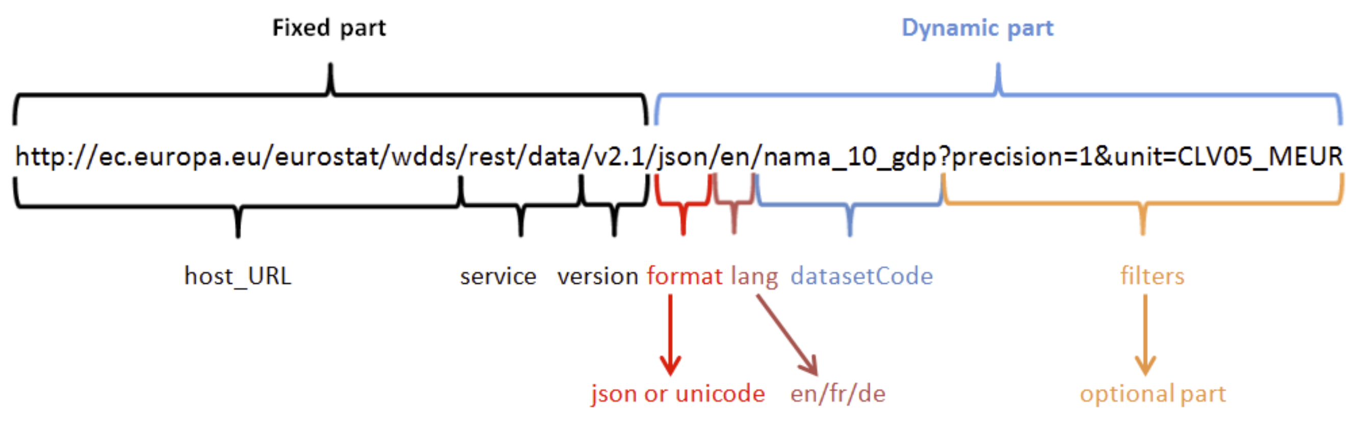
The picture below displays two things that we need to define to use the API. First, the “fixed part” (meaning the URL we use to call on Eurostat in general), and second, the “dynamic part” (which is the endpoint that we have to formulate to get the right data”)
26.1.1 Building the API request
Eurostat’s data is available from their servers. We could also have accessed these data through their old-fashioned database.
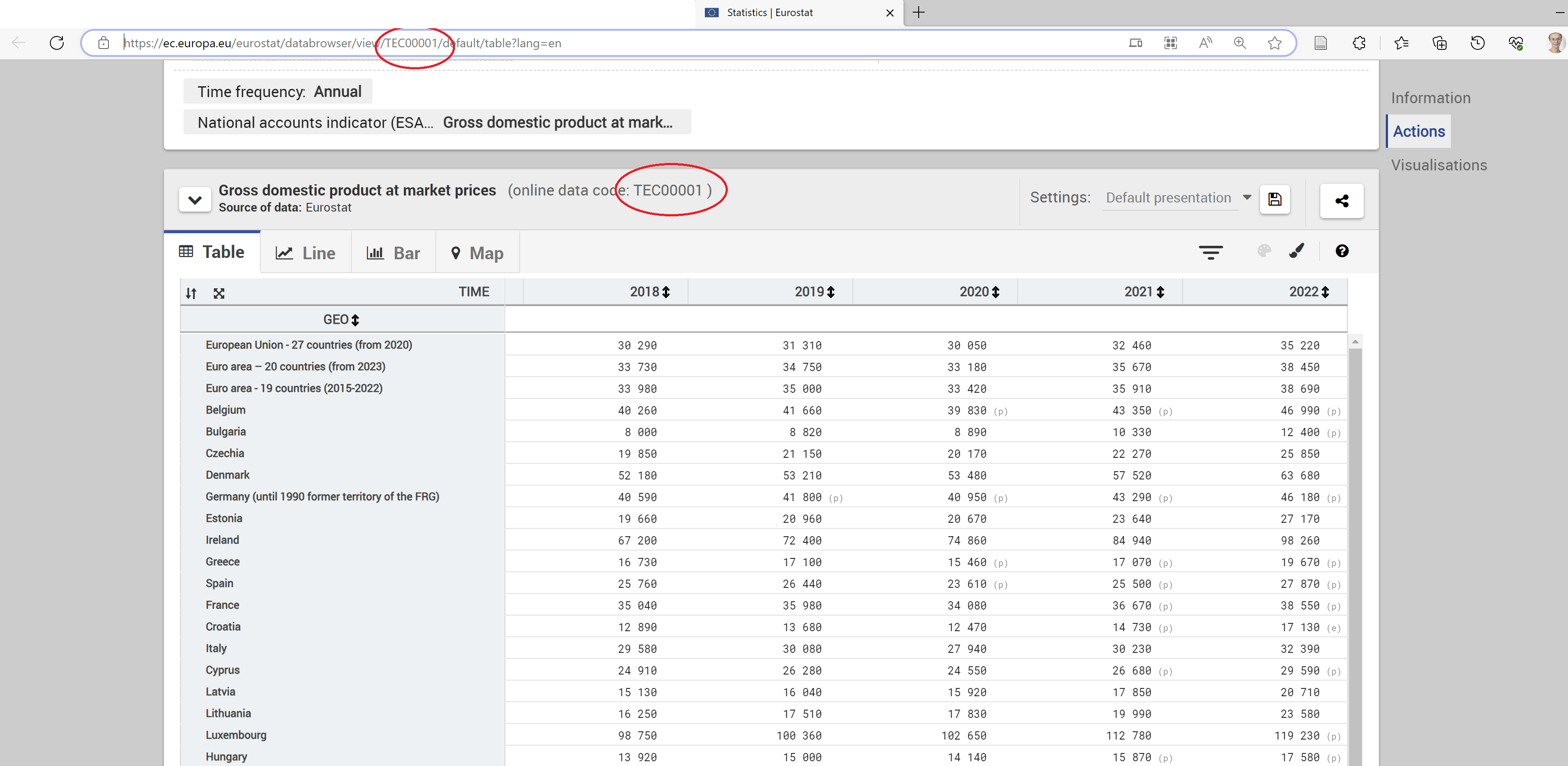
Because using the database to download data is manual, reduces reproducibility, makes data less timely and required local saving, we’ll extract the data through the API instead. When we want to extract data from the API, we need to be aware of a few things. First and foremost we want to know which dataset we want. Let’s assume we’re looking for data on GDP in European countries. Searching the Eurostat database, we find the Gross domestic product at market prices dataset. You can find the dataset here. The code in the end of this link, “TEC00001”, is the name of the dataset containing information on GDP in European countries.
Let’s try to fetch the GDP dataset using the API. Recall that an API request consists of a fixed part and an endpoint, and this is what we define in order to get what we want from the server. The endpoint is placed at the end of the host URL. Eurostat explains on their webpage that the fixed part (the host URL) for their API is:
https://ec.europa.eu/eurostat/api/dissemination/statistics/1.0/
We add the information we need to the end of this URL – thus making the endpoint.
What information do we need to add? The other things we need to know when making an API request to Eurostat, is:
- Which years we need data for: TIME
- Which units of observation (i.e. the countries or regions) we are interested in: GEO
- Which measure on the variable we’d like (dollars, percentages, etc.): UNIT
- Which variables we need (value added, individual consumption, GDP, etc.): NA_ITEM
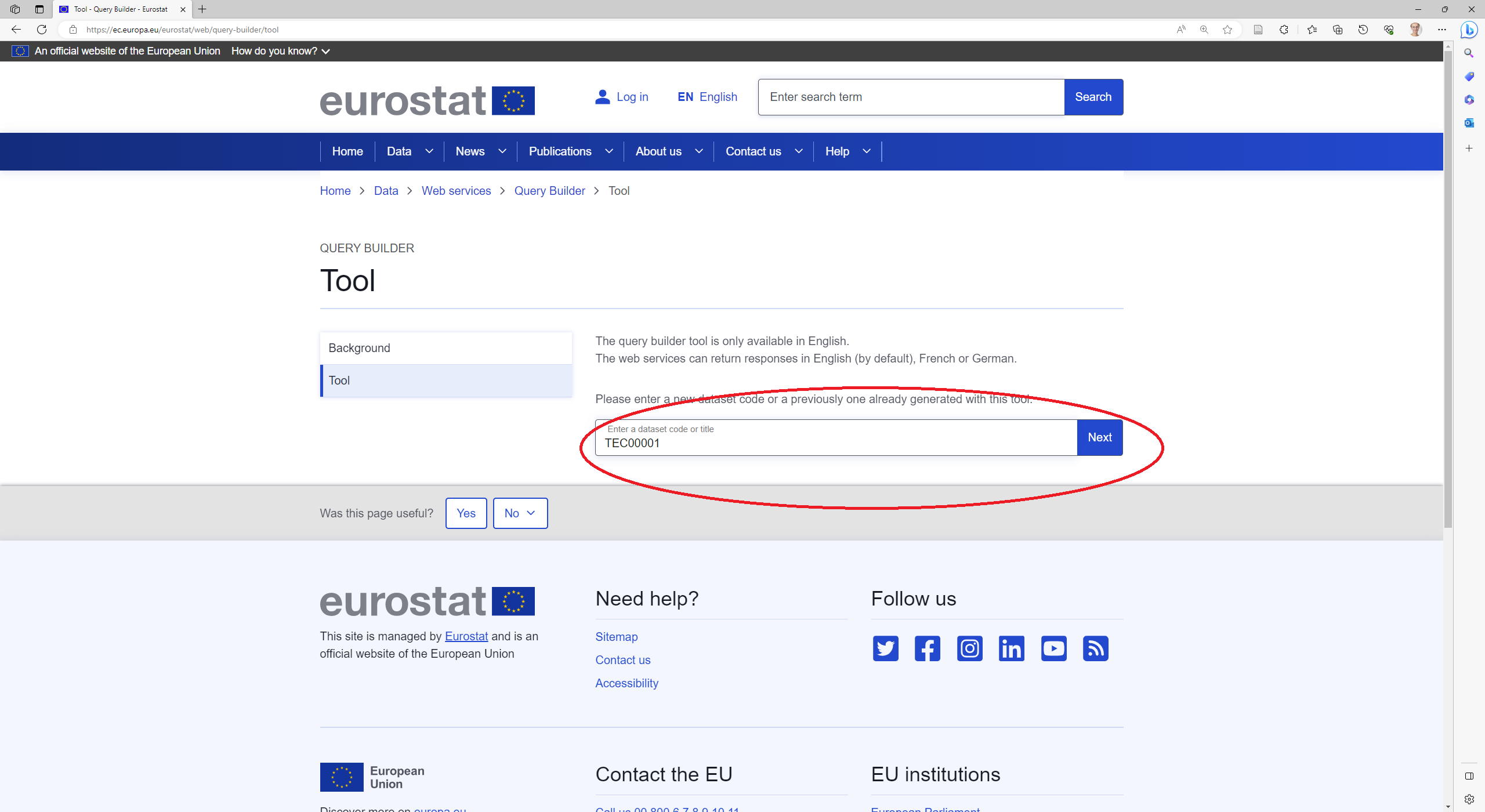
Let’s call these “dimensions”. We can find which dimensions we need to specify and how to specify them using the Eurostat query builder. To find the correct dataset in the query builder, paste the name of the dataset (found in the previous step) in the search bar.
Let’s say we want the dataset on GDP with:
- Value added, gross as the variable (NA_ITEM)
- Current prices, million euro as the measure (UNIT)
- For the country Belgium (GEO)
- For the years 2016 and 2017 (TIME)
Now we have a pretty specific wish, and this can be implemented into an API request. We specify this into the query builder by using the drop-down menus and clicking arrow that moves the relevant values for each dimension into ther right box. Remember to click from “Default” to “Static positions” in the radio-button choices. Then hit “Generate query”.
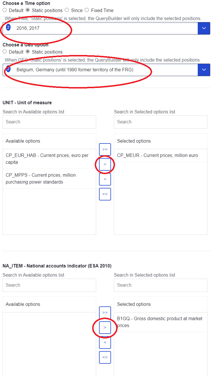
The link that comes out is the URL to the API request.
https://ec.europa.eu/eurostat/api/dissemination/statistics/1.0/data/tec00001?format=JSON&time=2016&time=2017&geo=BE&geo=DE&unit=CP_MEUR&na_item=B1GQ&lang=en
It contains the fixed part and the endpoint. As shown in the picture below, the endpoint contains all the information about which years to include, which countries to include, and so on. This is why it is the dynamic part – it is highly changeable depending on which dimensions we want to include.

If you try typing it into your browser and hit enter, it wil display the dataset there (in JSON format).
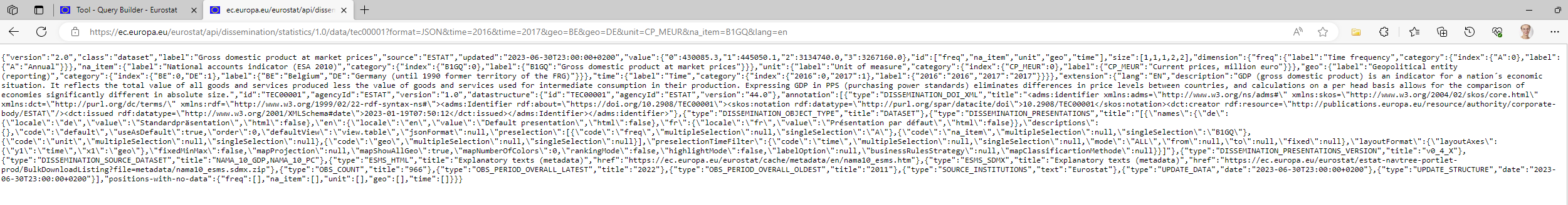
Notice how we, through the URL, specify the dataset, the na_item, the unit, the geo and the time.
26.1.2 Get the data into R
To get these data into R using the Eurostat API, we have to load the package httr, a package used to handle API requests. Then, we make an object of the URL request we just made.
library(httr)

url <- "https://ec.europa.eu/eurostat/api/dissemination/statistics/1.0/data/tec00001?format=JSON&time=2016&time=2017&geo=BE&geo=DE&unit=CP_MEUR&na_item=B1GQ&lang=en"
Second, we use the function GET from the package httr to make a GET request to the URL.
getresponse <- GET(url)

getresponse
Response [https://ec.europa.eu/eurostat/api/dissemination/statistics/1.0/data/tec00001?format=JSON&time=2016&time=2017&geo=BE&geo=DE&unit=CP_MEUR&na_item=B1GQ&lang=en]
Date: 2023-07-06 12:08
Status: 200
Content-Type: application/json
Size: 4.29 kBThe GET request contains various information on whether the call was successful, how long it took to make it, when it was made, and so on. This information might be useful, for example the status 200 means that the call was successful. A status of 400 (including 401, 402, 403, etc.) means that something went wrong, and the call was unsuccessful. You can read more about status codes here.
If the call was successful and everything is in order, we would ideally want the data. To extract the data from the object, we use the function content. Here, I specify the argument as to "text" to make a JSON-string out of the information.
json <- content(getresponse, as = "text")

json
[1] "{\"version\":\"2.0\",\"class\":\"dataset\",\"label\":\"Gross domestic product at market prices\",\"source\":\"ESTAT\",\"updated\":\"2023-07-05T23:00:00+0200\",\"value\":{\"0\":430085.3,\"1\":445050.1,\"2\":3134740.0,\"3\":3267160.0},\"id\":[\"freq\",\"na_item\",\"unit\",\"geo\",\"time\"],\"size\":[1,1,1,2,2],\"dimension\":{\"freq\":{\"label\":\"Time frequency\",\"category\":{\"index\":{\"A\":0},\"label\":{\"A\":\"Annual\"}}},\"na_item\":{\"label\":\"National accounts indicator (ESA 2010)\",\"category\":{\"index\":{\"B1GQ\":0},\"label\":{\"B1GQ\":\"Gross domestic product at market prices\"}}},\"unit\":{\"label\":\"Unit of measure\",\"category\":{\"index\":{\"CP_MEUR\":0},\"label\":{\"CP_MEUR\":\"Current prices, million euro\"}}},\"geo\":{\"label\":\"Geopolitical entity (reporting)\",\"category\":{\"index\":{\"BE\":0,\"DE\":1},\"label\":{\"BE\":\"Belgium\",\"DE\":\"Germany (until 1990 former territory of the FRG)\"}}},\"time\":{\"label\":\"Time\",\"category\":{\"index\":{\"2016\":0,\"2017\":1},\"label\":{\"2016\":\"2016\",\"2017\":\"2017\"}}}},\"extension\":{\"lang\":\"EN\",\"description\":\"GDP (gross domestic product) is an indicator for a nation´s economic situation. It reflects the total value of all goods and services produced less the value of goods and services used for intermediate consumption in their production. Expressing GDP in PPS (purchasing power standards) eliminates differences in price levels between countries, and calculations on a per head basis allows for the comparison of economies significantly different in absolute size.\",\"id\":\"TEC00001\",\"agencyId\":\"ESTAT\",\"version\":\"1.0\",\"datastructure\":{\"id\":\"TEC00001\",\"agencyId\":\"ESTAT\",\"version\":\"44.0\"},\"annotation\":[{\"type\":\"DISSEMINATION_DOI_XML\",\"title\":\"<adms:identifier xmlns:adms=\\\"http://www.w3.org/ns/adms#\\\" xmlns:skos=\\\"http://www.w3.org/2004/02/skos/core.html\\\" xmlns:dct=\\\"http://purl.org/dc/terms/\\\" xmlns:rdf=\\\"http://www.w3.org/1999/02/22-rdf-syntax-ns#\\\"><adms:Identifier rdf:about=\\\"https://doi.org/10.2908/TEC00001\\\"><skos:notation rdf:datatype=\\\"http://purl.org/spar/datacite/doi\\\">10.2908/TEC00001</skos:notation><dct:creator rdf:resource=\\\"http://publications.europa.eu/resource/authority/corporate-body/ESTAT\\\"/><dct:issued rdf:datatype=\\\"http://www.w3.org/2001/XMLSchema#date\\\">2023-01-19T07:50:12</dct:issued></adms:Identifier></adms:identifier>\"},{\"type\":\"DISSEMINATION_OBJECT_TYPE\",\"title\":\"DATASET\"},{\"type\":\"DISSEMINATION_PRESENTATIONS\",\"title\":\"[{\\\"names\\\":{\\\"de\\\":{\\\"locale\\\":\\\"de\\\",\\\"value\\\":\\\"Standardpräsentation\\\",\\\"html\\\":false},\\\"en\\\":{\\\"locale\\\":\\\"en\\\",\\\"value\\\":\\\"Default presentation\\\",\\\"html\\\":false},\\\"fr\\\":{\\\"locale\\\":\\\"fr\\\",\\\"value\\\":\\\"Présentation par défaut\\\",\\\"html\\\":false}},\\\"descriptions\\\":{},\\\"code\\\":\\\"default\\\",\\\"useAsDefault\\\":true,\\\"order\\\":0,\\\"defaultView\\\":\\\"view.table\\\",\\\"jsonFormat\\\":null,\\\"preselection\\\":[{\\\"code\\\":\\\"freq\\\",\\\"multipleSelection\\\":null,\\\"singleSelection\\\":\\\"A\\\"},{\\\"code\\\":\\\"na_item\\\",\\\"multipleSelection\\\":null,\\\"singleSelection\\\":\\\"B1GQ\\\"},{\\\"code\\\":\\\"unit\\\",\\\"multipleSelection\\\":null,\\\"singleSelection\\\":null},{\\\"code\\\":\\\"geo\\\",\\\"multipleSelection\\\":null,\\\"singleSelection\\\":null}],\\\"preselectionTimeFilter\\\":{\\\"code\\\":\\\"time\\\",\\\"multipleSelection\\\":null,\\\"singleSelection\\\":null,\\\"mode\\\":\\\"ALL\\\",\\\"from\\\":null,\\\"to\\\":null,\\\"fixed\\\":null},\\\"layoutFormat\\\":{\\\"layoutAxes\\\":{\\\"y1\\\":\\\"time\\\",\\\"x1\\\":\\\"geo\\\"},\\\"fixedMinMax\\\":false,\\\"mapProjection\\\":null,\\\"mapShowAllGeo\\\":true,\\\"mapNumberOfColors\\\":0,\\\"rankingMode\\\":false,\\\"highlightMode\\\":false,\\\"labelOption\\\":null,\\\"businessRulesStrategy\\\":null,\\\"mapClassificartionMethode\\\":null}}]\"},{\"type\":\"DISSEMINATION_PRESENTATIONS_VERSION\",\"title\":\"v0_4_X\"},{\"type\":\"DISSEMINATION_SOURCE_DATASET\",\"title\":\"NAMA_10_GDP,NAMA_10_PC\"},{\"type\":\"ESMS_HTML\",\"title\":\"Explanatory texts (metadata)\",\"href\":\"https://ec.europa.eu/eurostat/cache/metadata/en/nama10_esms.htm\"},{\"type\":\"ESMS_SDMX\",\"title\":\"Explanatory texts (metadata)\",\"href\":\"https://ec.europa.eu/eurostat/estat-navtree-portlet-prod/BulkDownloadListing?file=metadata/nama10_esms.sdmx.zip\"},{\"type\":\"OBS_COUNT\",\"title\":\"966\"},{\"type\":\"OBS_PERIOD_OVERALL_LATEST\",\"title\":\"2022\"},{\"type\":\"OBS_PERIOD_OVERALL_OLDEST\",\"title\":\"2011\"},{\"type\":\"SOURCE_INSTITUTIONS\",\"text\":\"Eurostat\"},{\"type\":\"UPDATE_DATA\",\"date\":\"2023-07-05T23:00:00+0200\"},{\"type\":\"UPDATE_STRUCTURE\",\"date\":\"2023-07-05T23:00:00+0200\"}],\"positions-with-no-data\":{\"freq\":[],\"na_item\":[],\"unit\":[],\"geo\":[],\"time\":[]}}}"Now that we have a JSON-object, we have all the information we need. But in R, we usually prefer dataframes to JSON. To work with JSON objects, we load a package that allows us to work with JSON, for example rjstat. From this package, we use the function fromJSONstat to make the JSON-file into a dataframe.
library(rjstat)

df <- fromJSONstat(json)
head(df)
We now have a dataframe with six variables and four rows. And we know the gross value added for Belgium and Germany in 2016 and 2017, measured in current prices (million euro).
To get a grasp of how APIs work, you can play around the the Eurostat query builder and use the code below to look at the datasets being produced. If you are unsure what the code for the dataset is, you can always explore through the Eurostat database.
library(httr)
library(rjstat)

url <- "https://ec.europa.eu/eurostat/api/dissemination/statistics/1.0/data/tec00001?format=JSON&time=2016&time=2017&geo=BE&geo=DE&unit=CP_MEUR&na_item=B1GQ&lang=en" # Change this with your own API request

getresponse <- GET(url)

json <- content(getresponse, "text")

df <- fromJSONstat(json)
26.2 API formats
APIs often give us semi-structured data. The formats are typically either JSON or XML, though you do see some APIs providing data in CSV-format as well. Let’s take a brief look at how to interpret these data formats.
Let’s say we have the dataset that we exctacted above – the dataset on Germany’s and Belgium’s gross value added measured in million euro, in 2016 and 2017. For a standard (structured) dataframe, this dataset looks like this:
It’s a dataframe with five variables and two rows.
In JSON, the structure of this dataset would be quite different. JSON works with so-called “key-value” pairs, which you can think of like specifying the group, and then specifying the variable in this group. They come in curly brackets {}, so you have a structure like:
{“key”: “value”}
For example:
{“name”: “Hannah”} {“city”: “Bergen”}
In the square brackets [] you usually have the values of the variable. The hierarchical structure is given by indents and brackets.
{
  "version": "2.0",
  "class": "dataset",
  "label": "Number of enterprises in the non-financial business economy by size class of employment",
  "source": "ESTAT",
  "updated": "2023-03-15T23:00:00+0100",
  "value": {
    "0": 611708,
    "1": 2467686,
    "2": 631819,
    "3": 2504371
  },
  "id": [
    "freq",
    "indic_sb",
    "nace_r2",
    "time",
    "geo",
    "size_emp"
  ],
  "size": [
    1,
    1,
    1,
    2,
    2,
    1
  ],
  "dimension": {
    "freq": {
      "label": "Time frequency",
      "category": {
        "index": {
          "A": 0
        },
        "label": {
          "A": "Annual"
        }
      }
    },
    "indic_sb": {
      "label": "Economical indicator for structural business statistics",
      "category": {
        "index": {
          "V11110": 0
        },
        "label": {
          "V11110": "Enterprises - number"
        }
      }
    },
    "nace_r2": {
      "label": "Statistical classification of economic activities in the European Community (NACE Rev. 2)",
      "category": {
        "index": {
          "B-N_S95_X_K": 0
        },
        "label": {
          "B-N_S95_X_K": "Total business economy; repair of computers, personal and household goods; except financial and insurance activities"
        }
      }
    },
    "time": {
      "label": "Time",
      "category": {
        "index": {
          "2016": 0,
          "2017": 1
        },
        "label": {
          "2016": "2016",
          "2017": "2017"
        }
      }
    },
    "geo": {
      "label": "Geopolitical entity (reporting)",
      "category": {
        "index": {
          "BE": 0,
          "DE": 1
        },
        "label": {
          "BE": "Belgium",
          "DE": "Germany (until 1990 former territory of the FRG)"
        }
      }
    },
    "size_emp": {
      "label": "Size classes in number of persons employed",
      "category": {
        "index": {
          "TOTAL": 0
        },
        "label": {
          "TOTAL": "Total"
        }
      }
    }
  }
}
XML-formats use tags to store information. As you can see, it’s quite similar to HTML. The variable group is defined by the less-and-greater-than signs < and >, and the end of a tag has a slash before the name of the tag. The hierarchical structure is given by the number of indents. To work with XML-formats in R, you can use the package xml. The functions xmlParse and xmlToList should give you dataframes from the XML.
<?xml version="1.0" encoding="UTF-8" ?>
<root>
  <version>2.0</version>
  <class>dataset</class>
  <label>Number of enterprises in the non-financial business economy by size class of employment</label>
  <source>ESTAT</source>
  <updated>2023-03-15T23:00:00+0100</updated>
  <value>
    <0>611708</0>
    <1>2467686</1>
    <2>631819</2>
    <3>2504371</3>
  </value>
  <id>freq</id>
  <id>indic_sb</id>
  <id>nace_r2</id>
  <id>time</id>
  <id>geo</id>
  <id>size_emp</id>
  <size>1</size>
  <size>1</size>
  <size>1</size>
  <size>2</size>
  <size>2</size>
  <size>1</size>
  <dimension>
    <freq>
      <label>Time frequency</label>
      <category>
        <index>
          <A>0</A>
        </index>
        <label>
          <A>Annual</A>
        </label>
      </category>
    </freq>
    <indic_sb>
      <label>Economical indicator for structural business statistics</label>
      <category>
        <index>
          <V11110>0</V11110>
        </index>
        <label>
          <V11110>Enterprises - number</V11110>
        </label>
      </category>
    </indic_sb>
    <nace_r2>
      <label>Statistical classification of economic activities in the European Community (NACE Rev. 2)</label>
      <category>
        <index>
          <B-N_S95_X_K>0</B-N_S95_X_K>
        </index>
        <label>
          <B-N_S95_X_K>Total business economy; repair of computers, personal and household goods; except financial and insurance activities</B-N_S95_X_K>
        </label>
      </category>
    </nace_r2>
    <time>
      <label>Time</label>
      <category>
        <index>
          <2016>0</2016>
          <2017>1</2017>
        </index>
        <label>
          <2016>2016</2016>
          <2017>2017</2017>
        </label>
      </category>
    </time>
    <geo>
      <label>Geopolitical entity (reporting)</label>
      <category>
        <index>
          <BE>0</BE>
          <DE>1</DE>
        </index>
        <label>
          <BE>Belgium</BE>
          <DE>Germany (until 1990 former territory of the FRG)</DE>
        </label>
      </category>
    </geo>
    <size_emp>
      <label>Size classes in number of persons employed</label>
      <category>
        <index>
          <TOTAL>0</TOTAL>
        </index>
        <label>
          <TOTAL>Total</TOTAL>
        </label>
      </category>
    </size_emp>
  </dimension>
</root>
And if you have a CSV, you can for example use read_csv to get it into R .
26.3 Nested dataframes
The JSON and XML formats contain some extra information – a bit of metadata on the dataset. They tell us the version of the dataset, the name of the dataset, the source, the date it was updated, and so on. And, nested into this information is the information on the dimensions. For something to be nested means that it basically becomes and undercategory of something else. You can think of it as a tree structure. The nested structure in the JSON and XML above looks something like this:
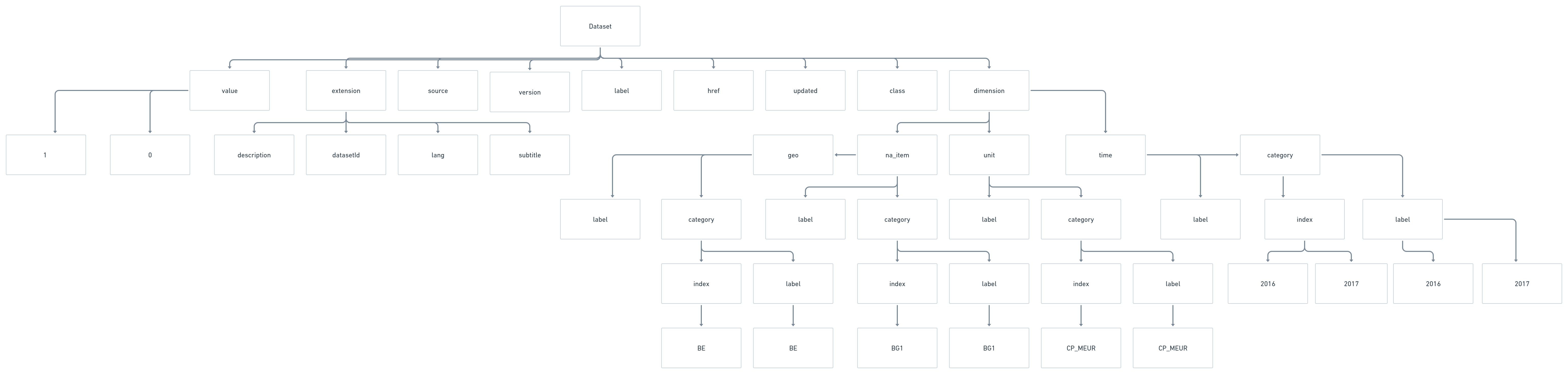
Sometimes, we’d like to keep the nested format in R. For example, maybe you have a category “countries”. Under that category you have categories for “Belgium”, “France”, “Germany” and so forth, and below that, data for GDP, population size and so forth. It is possible to keep the nested structure in R by creating nested dataframes. You can create your own nested dataframes by using the function nest, and then you can make them back to normal dataframes by using the function unnest. Below is an example of how you can read the full nested structure of a JSON-file into an R nested dataframe, and then unnest it.
library(jsonlite)

nested_df <- fromJSON("../datafolder/jsonexample.json", flatten = TRUE)

nested_df %>%
  unnest()
# A tibble: 4 × 26
version label href source updated class id size extension.datasetId
<chr> <chr> <chr> <chr> <chr> <chr> <chr> <int> <chr>
1 2.0 GDP and ma… http… Euros… 2022-0… data… unit 1 nama_10_gdp
2 2.0 GDP and ma… http… Euros… 2022-0… data… na_i… 1 nama_10_gdp
3 2.0 GDP and ma… http… Euros… 2022-0… data… geo 1 nama_10_gdp
4 2.0 GDP and ma… http… Euros… 2022-0… data… time 2 nama_10_gdp
# ℹ 17 more variables: extension.lang <chr>, value.0 <dbl>, value.1 <dbl>,
# dimension.unit.label <chr>, dimension.unit.category.index.CP_MEUR <int>,
# dimension.unit.category.label.CP_MEUR <chr>, dimension.na_item.label <chr>,
# dimension.na_item.category.index.B1G <int>,
# dimension.na_item.category.label.B1G <chr>, dimension.geo.label <chr>,
# dimension.geo.category.index.BE <int>,
# dimension.geo.category.label.BE <chr>, dimension.time.label <chr>, …27 R-packages for API requests
If you thought gathering data through the Eurostat API was cumbersome, you are not the first one to think that. Using APIs through the httr package is alright, but it can be quite tricky to get into sometimes. That is why, luckily, many package builders in the R community have created their own packages to use APIs easily in R. A quick search on the internet tells us that someone have created an R package for the Eurostat API as well!
The package is called eurostat. Remember, the first time you use a package you have to install.packages(). After that, we can load it into R.
library(eurostat)Warning: package 'eurostat' was built under R version 4.2.3The package has many useful functions. get_eurostat_toc, for example, gives us a table of contents for the eurostat databases. Here, we can browse to find datasets useful for our analysis.
get_eurostat_toc() %>%
  head() # Displays the first six rows of the dataset
# A tibble: 6 × 8
title code type `last update of data` last table structure…¹ `data start`
<chr> <chr> <chr> <chr> <chr> <chr>
1 Databas… data fold… <NA> <NA> <NA>
2 General… gene… fold… <NA> <NA> <NA>
3 Europea… euro… fold… <NA> <NA> <NA>
4 Balance… ei_bp fold… <NA> <NA> <NA>
5 Current… ei_b… data… 04.07.2023 04.07.2023 1992Q1
6 Financi… ei_b… data… 04.07.2023 04.07.2023 1992Q1
# ℹ abbreviated name: ¹`last table structure change`
# ℹ 2 more variables: `data end` <chr>, values <chr>With the function search_eurostat, we can search for datasets for specific keywords. Using this function, we see that our dataset nama_10_gdp comes high up on the list.
search_eurostat("GDP") %>%
  head()
# A tibble: 6 × 8
title code type `last update of data` last table structure…¹ `data start`
<chr> <chr> <chr> <chr> <chr> <chr>
1 GDP and… nama… data… 05.07.2023 16.02.2023 1975
2 GDP and… namq… data… 05.07.2023 27.04.2023 1975Q1
3 Gross d… nama… data… 21.02.2023 19.02.2023 2000
4 Average… nama… data… 21.02.2023 19.02.2023 2000
5 Gross d… nama… data… 21.02.2023 19.02.2023 2000
6 Gross d… nama… data… 11.04.2023 20.02.2023 1995
# ℹ abbreviated name: ¹`last table structure change`
# ℹ 2 more variables: `data end` <chr>, values <chr>To get the data into R, we use the function get_eurostat.
get_eurostat("tec00001") %>%
  head()
# A tibble: 6 × 5
na_item unit geo time values
<chr> <chr> <chr> <date> <dbl>
1 B1GQ CP_EUR_HAB AL 2011-01-01 3190
2 B1GQ CP_EUR_HAB AT 2011-01-01 36970
3 B1GQ CP_EUR_HAB BE 2011-01-01 34060
4 B1GQ CP_EUR_HAB BG 2011-01-01 5640
5 B1GQ CP_EUR_HAB CH 2011-01-01 65190
6 B1GQ CP_EUR_HAB CY 2011-01-01 23340And indeed, you can filter in the R-code just like we did above in the URL by adding the argument filter and wrap the filters into a list. To learn more about how to use the Eurostat API R-package, take a look at this link.
get_eurostat("tec00001",
             filters = list(na_item = "B1GQ",
                            unit = "CP_MEUR",
                            geo = c("BE", "DE"),
                            time = c("2016", "2017"))) %>%
  head()
Reading cache file C:\Users\solvebjo\AppData\Local\Temp\RtmpOg6QVg/eurostat/tec00001_date_code_FF.rdsTable tec00001 read from cache file: C:\Users\solvebjo\AppData\Local\Temp\RtmpOg6QVg/eurostat/tec00001_date_code_FF.rds# A tibble: 4 × 6
freq na_item unit geo time values
<chr> <chr> <chr> <chr> <date> <dbl>
1 A B1GQ CP_MEUR BE 2016-01-01 430085.
2 A B1GQ CP_MEUR BE 2017-01-01 445050.
3 A B1GQ CP_MEUR DE 2016-01-01 3134740
4 A B1GQ CP_MEUR DE 2017-01-01 3267160