library(tidyverse)

costofliving <- read_rds("../datafolder/costofliving2.rds")17 Descriptive measures
Descriptive statistics are useful in giving insights about patterns in your data. We are not going to delve heavily into statistics in this course, but we’ll look at a few basic measures, including finding the:
meanmedianmodevariancestandard deviationcount
of a variable.
Let’s read the dataset from yesterday in to R.
17.1 Central tendency
First, we’ll look at measures to find central tendency. These measures reflect the center of a data distribution. What is a distribution, you might ask. Well, it’s simply how our data looks with regard to how many different units have different values. For example, say our variable is how many minutes a person spends in the shower. If most people in the datset spends about 10 minutes, while a bit few spend equally 5 minutes and 15 minutes, we’d get a symmetrical distribution. However, if relatively more people spend 15 minutes, we’ll get a negative skew, which means that the distribution would lean right. This is important because how the data is distributed is fundamental to a lot of techniques and models we use.
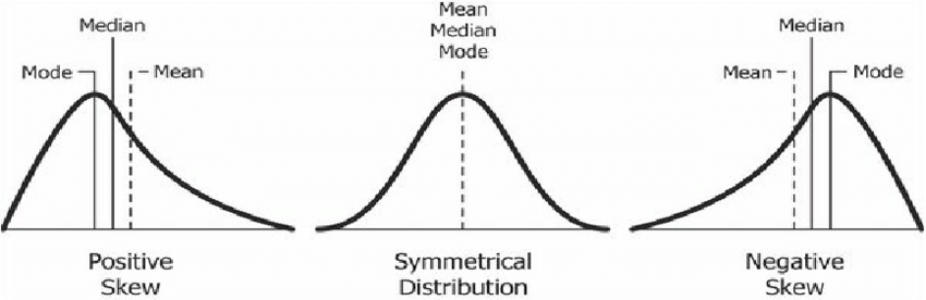
We’ll look more into plotting in week 2. For now, I visualize the distribution of the cofi variable by making a histogram. Looks most cities here have a cost of living around 70. There’s a slight negative skew to the data, meaning that most cities (thankfully) have a cost of living lower to that of New York.
costofliving %>%
  ggplot(aes(cofi)) +
  geom_histogram() +
  ggtitle("Distibution of cost of living")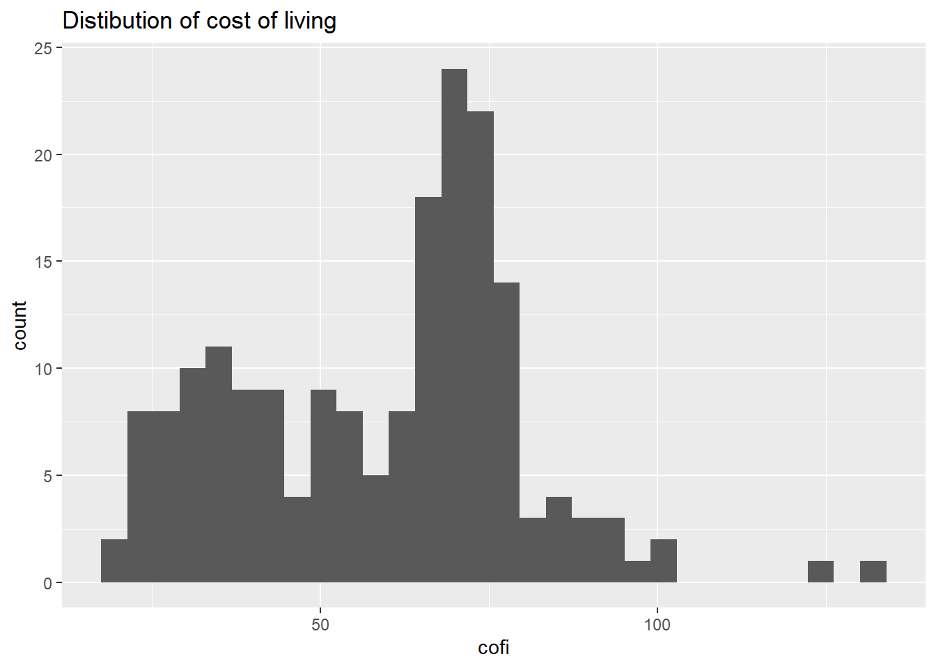
Measures of central tendency, then, tells us where most of the units fall. There are three main ways of measuring central tendency:
- Mean: the sum of the values divided by the number of values.
- Median: the value that’s exactly in the middle of the data when it is ordered.
- Mode: the number which appears most often.
Notice from the figure above that if the distribution is skewed, the mean, the median and the mode will differ. We’ll find the mean, median and mode of our variable cofi. First, we load the tidyverse package.
library(tidyverse)Then, finding the mean, we can use summarise together with the mean function. Notie that we add na.rm = TRUE, which means that R should calculate the mean without taking into account that there are missing values in the data. If there are missing values and we do not set na.rm to TRUE, the mean would become NA.
costofliving %>%
  summarise(cofi_mean = mean(cofi, na.rm = TRUE)) # Use summarise and mean on the variable, set na.rm to TRUE
# A tibble: 1 × 1
cofi_mean
<dbl>
1 58.7The average cost of living in all the cities in our dataset is 57.44.
To calculate the median, use the same procedure with summarise, but use the function median. Remember to add na.rm = TRUE to this piece of code as well.
costofliving %>%
  summarise(cofi_median = median(cofi, na.rm = TRUE)) # Use summarise and median on the variable, set na.rm to TRUE
# A tibble: 1 × 1
cofi_median
<dbl>
1 64.4The median is slightly higher than the mean, which makes sense since our data has a negative skew.
Lastly, the mode is the value that occurs most frequently in our data. It can be a good measure if you have a count variable (i.e. a variable where you for example have counted the number of times a person goes to the cinema), but in cases where you have continuous data with decimals, it’s usually not that useful to see which value that is most frequent. Thus, here, we calculate the mode on the country variable to see which country appears most often.
costofliving %>%
  count(country, name = "number_of_countries") %>% # Count the number of times each country shows up, giving the count variable the name number_of_countries
  slice_max(number_of_countries, n = 1) # Picking out the first maximum value of the number_of_countries variable
# A tibble: 1 × 2
country number_of_countries
<chr> <int>
1 United States 3517.2 Spread
Now that we know where most of the units fall on the distribution, it would also be useful to know something about the units that are not “typical” for the data. This is often referred to as the spread of the data, because it tells us something about all the units that fall around the central tendency.
Two measures are typically used:
- Variance: How much a variable varies around the mean.
- Standard deviation: How far on average each value lies from the mean.
To calculate the variance, use var. Admittedly, the variance measure does not tell us much except that there is variation around the mean in our data.
costofliving %>%
  summarise(cofi_variance = var(cofi, na.rm = TRUE)) # A positive number tells us that there is variation in our data
# A tibble: 1 × 1
cofi_variance
<dbl>
1 439.To say something more substantive about the spread, we can use the standard deviation. To calculate this, use the sd function. This is a measure that occurs in the same scale as the variable, so the standard deviation is the average units around the mean.
costofliving %>%
  summarise(cofi_sd = sd(cofi, na.rm = TRUE)) # Units vary on average 21.63 cost of living index points around the mean of 57.44.
# A tibble: 1 × 1
cofi_sd
<dbl>
1 21.017.3 Count
If we have a categorical variable, it does not make sense to find either the mean, median, variance or standard deviation because there are no numerical values to calculate these statistics from. In these cases, we often just count the number of times different values occur.
We already had a look at this with calculating the mode. Here, I use somewhat of the same procedure by using group_by and count. I leave out the slice_max function which grabs only parts of the rows, and use instead arrange and desc to get the variable in descending order.
costofliving %>%
  group_by(country) %>% # Find the next statistic per country
  count(name = "country_n") %>% # Count the number of instances (i.e. the number of countries per city)
  arrange(desc(country_n)) # Arrange in descending order so that the highest values come on top
# A tibble: 65 × 2
# Groups: country [65]
country country_n
<chr> <int>
1 United States 35
2 India 16
3 United Kingdom 14
4 Germany 12
5 Canada 6
6 Italy 5
7 Australia 4
8 Netherlands 4
9 Poland 4
10 Spain 4
# ℹ 55 more rowsAlternatively, we could find the percentages. Here, I find how many cities in the dataset each country in percentage stand for. Almost 19 percent of the cities in our dataset are in the United States.
all_countries <- costofliving %>%
  count(name = "all_countries") %>%
  pull() # Fetch the value from the dataset, creating a vector

costofliving %>%
  group_by(country) %>%
  count(name = "country_n") %>%
  ungroup() %>%
  mutate(country_percentage = country_n/all_countries * 100) %>% # Make a new variable calculating the percentage, i.e. the count divided by the total multiplied by 100
  arrange(desc(country_percentage))
# A tibble: 65 × 3
country country_n country_percentage
<chr> <int> <dbl>
1 United States 35 18.7
2 India 16 8.56
3 United Kingdom 14 7.49
4 Germany 12 6.42
5 Canada 6 3.21
6 Italy 5 2.67
7 Australia 4 2.14
8 Netherlands 4 2.14
9 Poland 4 2.14
10 Spain 4 2.14
# ℹ 55 more rows