33 Text vectorization
Once we have tokenized the text and done the last bit of preprocessing, we are ready to vectorize the text. Text vectorization involves converting the text into a numerical representation. Once again, we have several options, but in this class we’ll focus on two of the easiest; bag of words and TF-IDF.
33.1 Bag of words
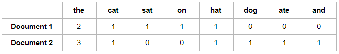
Imagine that you take all the documents that you’re analyzing, count how many times every single word shows up in the document, and put it into a matrix. This is bag of words. It’s a matrix with documents as the rows and words as the columns. In our case, the rows would have been songnames. This means that when we create a matrix with bag of words, the matrices become very big (wide). We have 14 songs, but hundreds of words.
library(quanteda)Warning: package 'quanteda' was built under R version 4.2.3Package version: 3.3.1
Unicode version: 13.0
ICU version: 69.1Parallel computing: 16 of 16 threads used.See https://quanteda.io for tutorials and examples.library(tidytext)Warning: package 'tidytext' was built under R version 4.2.3library(tidyverse)Warning: package 'ggplot2' was built under R version 4.2.3Warning: package 'tibble' was built under R version 4.2.3Warning: package 'dplyr' was built under R version 4.2.3── Attaching core tidyverse packages ──────────────────────── tidyverse 2.0.0 ──
✔ dplyr 1.1.2 ✔ readr 2.1.4
✔ forcats 1.0.0 ✔ stringr 1.5.0
✔ ggplot2 3.4.2 ✔ tibble 3.2.1
✔ lubridate 1.9.2 ✔ tidyr 1.3.0
✔ purrr 1.0.1 ── Conflicts ────────────────────────────────────────── tidyverse_conflicts() ──
✖ dplyr::filter() masks stats::filter()
✖ dplyr::lag() masks stats::lag()
ℹ Use the conflicted package (<http://conflicted.r-lib.org/>) to force all conflicts to become errorsTo exemplify the process, let’s pick three sentences from our songs and put them into a matrix. As you can see, the matrix quickly expands as we add text. Here, we can also see the benefits of preprocessing the text – we could avoid quite a bit of noise if we remove the stopwords before vectorizing.
| Sentence | you | were | in | love | or | so | said | i | know | boat | a | can | get | on | she | isn’t | merely | insane |
|---|---|---|---|---|---|---|---|---|---|---|---|---|---|---|---|---|---|---|
| you were in love or so you said | 2 | 1 | 1 | 1 | 1 | 1 | 1 | 0 | 0 | 0 | 0 | 0 | 0 | 0 | 0 | 0 | 0 | 0 |
| i know a boat you can get on | 1 | 0 | 0 | 0 | 0 | 0 | 0 | 1 | 1 | 1 | 1 | 1 | 1 | 1 | 0 | 0 | 0 | 0 |
| she isn’t in love she’s merely insane | 0 | 0 | 1 | 1 | 0 | 0 | 0 | 0 | 0 | 0 | 0 | 0 | 0 | 0 | 1 | 1 | 1 | 1 |
How to create a bag of words in R? One possibility is to use the quanteda package and the function cast_dfm. To do this, we first need to count the number of times each words shows up in each song, as we’ve done before. Here, I also show how to use name = "count" to call the new variable “count”. Then use cast_dfm, and as arguments, we specify (1) the documents to be the rows, (2) the tokens to be the columns and (3) the number to fill the cells. dfm stands for document feature matrix.
westside_tokens %>%
  count(songname, stem, name = "count") %>% # By default, the count-variable is called "n". Use name = "" to change it.
  cast_dfm(songname, # Specify the douments in your analysis (becoming the rows)
           stem, # Specify the tokens in your analysis (becoming the columns)
           count) # Specify the number of times each token shows up in each document (becoming the cells)
Document-feature matrix of: 14 documents, 444 features (91.09% sparse) and 0 docvars.
features
docs anita belong boi brother care forev forget head
a-boy-like-thati-have-a-love 1 1 1 1 1 1 1 1
america 0 0 0 0 0 0 0 0
cool 0 0 1 0 0 0 0 0
finale 0 0 0 0 0 0 0 0
gee-officer-krupke 0 0 1 1 1 0 0 1
i-feel-pretty 0 0 1 0 0 0 0 0
features
docs hear heart
a-boy-like-thati-have-a-love 1 1
america 0 0
cool 0 0
finale 0 0
gee-officer-krupke 0 0
i-feel-pretty 0 0
[ reached max_ndoc ... 8 more documents, reached max_nfeat ... 434 more features ]33.2 TF-IDF
Bag of words work surprisingly well for being such a crude way of vectorizing, but it definitely has its limits. For example, it does nothing to try to convey how important a specific word is at representing the text. In the sentence: “Democracy is under attack”, most of us would agree that the words “democracy” and “attack” are more important to the meaning of the sentence than “is” and “under”. However, a bag of words technique would weigh all words equally, and this technique might give too much weight to unimportant words, since these tend to show up more often than important words.
To account for this, we introduce a way of weighing the words. This technique gives more weight to words that occur rather frequently in a text compared to how often the word occurs in other texts in our selection. Thus, we assume that words occurring frequently in a text compared to other texts will carry more meaning as to what the text is about. Words occurring frequently in all texts – such as “under” and “before” – are given less weight. The weighing mechanism is called term frequency - inverse document frequency, shortened TF-IDF.
Basically, the TF-IDF measure counts the number of times a given term shows up in a document (term frequency), and divides it by a measure showing how frequent the term is in the selection of documents overall (inverse document frequency)1.
\(TF-IDF = \frac{TermFrequency}{InverseDocumentFrequency}\)
To do calculate the TF-IDF in R, we can use the function bind_tf_idf from the tidytext package. This gives us both the term frequency (tf), the inverse document frequency (idf) and the term frequency inverse document frequency (tf-idf) for every token in the texts.
westside_tokens <- westside_tokens %>%
  count(songname, stem, name = "count") %>%
  bind_tf_idf(stem, songname, count) # Making the tf-idf measure

westside_tokens
# A tibble: 554 × 6
songname stem count tf idf tf_idf
<chr> <chr> <int> <dbl> <dbl> <dbl>
1 a-boy-like-thati-have-a-love anita 1 0.0333 2.64 0.0880
2 a-boy-like-thati-have-a-love belong 1 0.0333 2.64 0.0880
3 a-boy-like-thati-have-a-love boi 1 0.0333 1.03 0.0343
4 a-boy-like-thati-have-a-love brother 1 0.0333 1.54 0.0513
5 a-boy-like-thati-have-a-love care 1 0.0333 1.54 0.0513
6 a-boy-like-thati-have-a-love forev 1 0.0333 1.95 0.0649
7 a-boy-like-thati-have-a-love forget 1 0.0333 1.95 0.0649
8 a-boy-like-thati-have-a-love head 1 0.0333 1.95 0.0649
9 a-boy-like-thati-have-a-love hear 1 0.0333 2.64 0.0880
10 a-boy-like-thati-have-a-love heart 1 0.0333 1.95 0.0649
# ℹ 544 more rowsWe can also plot these tf-idf weighed tokens as we did above. Although the difference is not glaring in this case because we do not have that much text to work with, we can for example notice that the word “boi” (“boy”) has gotten a lower weight since it shows up frequently in several different songs.
plot_df_tfidf <- westside_tokens %>%
  group_by(songname) %>%
  slice_max(tf_idf, n = 5) %>% # Get the five highest units on the tf-idf measure
  ungroup()

plot_df_tfidf %>%
  ggplot(aes(tf_idf, fct_reorder(stem, tf_idf), # Plotting words based on their tf-idf score
             fill = songname)) +
  geom_bar(stat = "identity") +
  facet_wrap(~ songname, ncol = 4, scales = "free") +
  labs(x = "", y = "") +
  theme_bw() +
theme(legend.position = "none") 
And we can create a document feature matrix (dfm) using tf-idf instead of bag of words.
westside_tokens %>%
  cast_dfm(songname,
           stem,
           tf_idf) # Specify tf-idf
Document-feature matrix of: 14 documents, 444 features (91.09% sparse) and 0 docvars.
features
docs anita belong boi brother
a-boy-like-thati-have-a-love 0.08796858 0.08796858 0.03432065 0.05134817
america 0 0 0 0
cool 0 0 0.04290081 0
finale 0 0 0 0
gee-officer-krupke 0 0 0.00837089 0.01252394
i-feel-pretty 0 0 0.01687901 0
features
docs care forev forget head
a-boy-like-thati-have-a-love 0.05134817 0.06486367 0.06486367 0.06486367
america 0 0 0 0
cool 0 0 0 0
finale 0 0 0 0
gee-officer-krupke 0.01252394 0 0 0.01582041
i-feel-pretty 0 0 0 0
features
docs hear heart
a-boy-like-thati-have-a-love 0.08796858 0.06486367
america 0 0
cool 0 0
finale 0 0
gee-officer-krupke 0 0
i-feel-pretty 0 0
[ reached max_ndoc ... 8 more documents, reached max_nfeat ... 434 more features ]saveRDS(westside_tokens, file = "../datafolder/westside_tokens.rds")The inverse document frequency measure for any term is calculated as \(idf(term) = ln(\frac{n_{Documents}}{n_{DocumentsContainingTerm}})\)↩︎